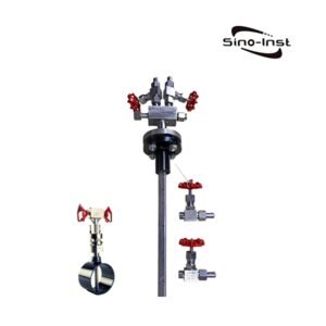
Flow Rate and Pressure: Formula, Worked Example & Conversion Table

Flow rate and pressure are linked by Bernoulli’s equation, by friction losses, and by the geometry of whatever the fluid passes through. A pump that delivers 200 kPa across a 50 mm pipe will not push the same volume per minute as one delivering 200 kPa across a 25 mm pipe. Pressure alone is not flow — and flow alone is not pressure. The rest of this page walks through the formulas you actually use in the field, two worked examples, and the corrections every engineer needs to apply when reading a flow meter spec from a vendor.

Contents

How Flow Rate and Pressure Relate

Pressure is the energy per unit volume that drives a fluid; flow rate is how much volume crosses a section in a given time. They are tied by three physical realities:

  • Energy conservation. Bernoulli’s equation says total head — pressure + velocity + elevation — is conserved along a streamline (ideal case). Drop the pressure across an orifice and the velocity (hence flow) rises.
  • Friction loss. Real pipes consume pressure to push the fluid against wall shear. Doubling the flow roughly quadruples the friction loss in turbulent flow.
  • Geometry. Pipe diameter, roughness, fittings, and the restriction itself (orifice, valve, nozzle) determine how much flow a given pressure differential produces.
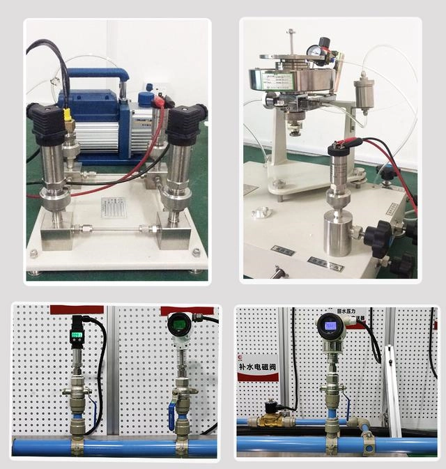
Pressure transmitter installation reading line pressure for flow calculation

The Five Core Formulas

Keep these five formulas on a card next to your desk. They cover 90% of plant calculations.

Use caseFormulaNote
Bernoulli (ideal)P + ½ρv² + ρgh = constantConservation along a streamline, no friction
Orifice / Venturi (incompressible)Q = Cd · A · √(2ΔP / ρ)The workhorse for DP-based flow measurement
Darcy-Weisbach (pipe friction)ΔP = f · (L/D) · (ρv²/2)Friction factor f from Moody chart
Hagen-Poiseuille (laminar flow)Q = (Π · ΔP · D⁴) / (128 · μ · L)Valid for Re < 2300; very small pipes/oils
Valve / restriction (Cv coefficient)Q = Cv · √(ΔP / SG)Flow in GPM, ΔP in psi, SG specific gravity

Two practical notes. The orifice formula uses ΔP (pressure differential), not absolute line pressure — a transmitter reporting 5 bar of line pressure tells you nothing about flow unless you also know the upstream-to-downstream drop. And the Cv formula is unit-bound: psi and GPM are required as input, not bar and m³/h. Convert before using or read our differential-pressure flow calculator walkthrough for a SI-unit version.

Worked Example — Calculating Flow from Pressure

An orifice plate sits in a 100 mm horizontal water line. Bore diameter is 60 mm. The DP transmitter reads 25 kPa. Find the flow rate.

If your pump curve is in LPM but the procurement spec is in US gallons per minute, run a sanity check on the conversion before sizing — our LPM to GPM conversion guide covers the US/UK gallon gap and the spec-sheet decoder.

  1. Beta ratio β = d/D = 60/100 = 0.6.
  2. For β = 0.6 in turbulent water flow, discharge coefficient Cd ≈ 0.62 (ISO 5167 table).
  3. Orifice area A = π · (0.06/2)² = 2.827 × 10⁻³ m².
  4. Water density ρ = 1000 kg/m³. ΔP = 25,000 Pa.
  5. Q = 0.62 · 2.827e-3 · √(2 · 25000 / 1000) = 0.62 · 2.827e-3 · 7.07 = 0.01239 m³/s.
  6. Convert to working units: 0.01239 m³/s × 3600 = 44.6 m³/h, or about 196 GPM.

The same 25 kPa drop across a different bore would give a different flow. That dependence on geometry is why DP flow meters need a calibration certificate that matches the installed bore and pipe, not just the spec sheet’s claimed accuracy. See straight-run pipe requirements for the installation rules that keep the calibration valid.

Pressure Drop in Real Piping

The total pressure loss in a real pipe run is the sum of friction in straight pipe plus losses at every fitting. A simplified working form:

  • Straight pipe loss: Darcy-Weisbach (above). Friction factor f rises with roughness and falls with Reynolds number.
  • Fitting losses: ΔPfitting = K · (ρv²/2). K values from tables — 90° elbow K ≈ 0.75, gate valve fully open K ≈ 0.15, sudden contraction K ≈ 0.5.
  • Elevation: ρgh — 1 m of water adds 9.81 kPa to the static head requirement.

The friction line on a pump curve is the sum of these terms. When the pump’s pressure output equals the system’s friction demand at a given flow, the system stabilises at that operating point. Most underperforming pump installations trace back to a friction estimate that ignored elbows, valves, or the eventual fouling-up of strainers and heat exchangers.

Why the Pressure-Flow Curve Matters for Pump Selection

A centrifugal pump produces more flow at lower pressure and less flow at higher pressure. Plot the pump’s pressure-vs-flow curve on the same axes as the system’s friction curve. The intersection is the operating point.

  • If the system curve drifts left of the pump’s best efficiency point (BEP), you waste energy and risk recirculation damage.
  • If the system curve sits right of BEP, the motor may overload during low-resistance conditions (filter clean, valve open).
  • Aim to size pumps so the design point sits within ±10% of BEP, then verify with a flow meter K-factor calibration after commissioning.

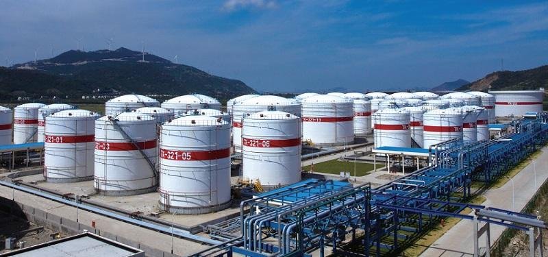
Quick Reference Table — Pressure to Flow

Approximate flow through a 1″ (25 mm) clean steel pipe, water at 20 °C, no fittings, fully developed turbulent flow. Use as a sanity check, not a design value.

Line pressure (psi)Approx. flow (GPM)Approx. flow (m³/h)
10143.2
20204.5
40286.4
60347.7
80409.1
1004410.0

Note the non-linearity. Doubling pressure does not double flow because friction losses scale with v² — about 40% more pressure is needed to move twice the volume. Engineers used to volumetric scaling are often surprised by how badly bigger pumps underperform expectations.

Common Mistakes Calculating Flow from Pressure

  • Confusing absolute pressure with differential pressure. Line pressure tells you nothing on its own — flow follows the DP across a known restriction.
  • Ignoring fluid properties. Hot water has a different viscosity and density from cold water. A static vs dynamic pressure check matters before reaching for Bernoulli.
  • Assuming the orifice Cd is 1.0. Real coefficients run 0.6 to 0.8 depending on beta ratio and Reynolds number. ISO 5167 lists actual values.
  • Mixing units. The Cv formula needs psi and GPM. The orifice formula needs SI units. Convert before substituting.
  • Forgetting upstream straight-run. An orifice that meets ISO 5167 in the lab but sits 1 D downstream of a 90° elbow on site will read 5-10% off true flow. Read the magnetic flow meter installation guide for similar straight-pipe rules across meter families.

Featured DP Flow Meters and Pressure Transmitters from Sino-Inst

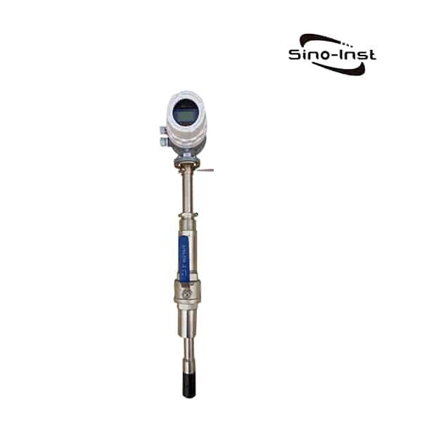
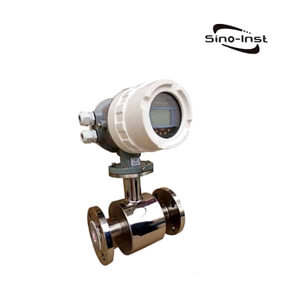
Industrial Magmeter Flow Meters

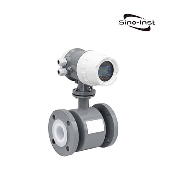
DN6-DN3000 | 4-20 mA, pulse, Modbus | conductive liquids — measures flow directly, no DP calculation needed.
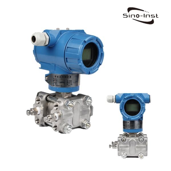
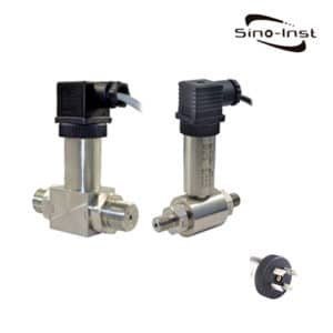
SMT3151DP Differential Pressure Transmitter

100:1 turndown | 0.075% accuracy | HART + 4-20 mA — pair with an orifice plate to compute Q from ΔP.

Verabar Averaging Pitot Tube

Insertion design | low permanent pressure loss | DP output for air, gas, steam, water — minimal installation cost.

Frequently Asked Questions

What is the formula for flow rate from pressure?

For a fluid passing through a restriction: Q = Cd · A · √(2ΔP / ρ). ΔP is the pressure drop across the restriction, A is the restriction area, ρ is the fluid density, and Cd is the discharge coefficient (typically 0.6 to 0.8 for orifices).

Does higher pressure always mean higher flow?

No. Higher line pressure does not by itself produce more flow. Flow rises when the pressure differential across the system increases, while the system geometry stays constant. A sealed pipe at 10 bar has zero flow despite high pressure.

How do I convert pressure to flow rate in GPM?

The simplest practical conversion uses the valve coefficient: Q (GPM) = Cv · √(ΔP / SG), where ΔP is in psi and SG is specific gravity. For pipes without a defined restriction, you need pipe length, diameter, roughness, and fluid properties — there is no single-number conversion.

What is Bernoulli’s equation used for?

Bernoulli’s equation conserves total energy (pressure + kinetic + potential) along a streamline for an ideal fluid. In instrumentation, it underpins the orifice, venturi, and pitot-tube flow-measurement formulas. Real-world calculations correct Bernoulli with a discharge coefficient or friction term.

Why does my flow meter read low at high pressure?

Several causes. A DP meter on an orifice reads correctly only within its calibrated turndown — extreme pressure drops outside that range introduce nonlinearity. Or the pressure is compressing a gas, so volumetric flow shrinks even though mass flow is steady. Check the meter’s calibration certificate and whether the reading is volumetric or mass-based.

Sino-Inst engineers have specified flow elements, DP transmitters, and magnetic and ultrasonic flow meters for refineries, water utilities, and chemical sites across more than 50 countries. Send the line size, fluid properties, and the pressure range — the team will return a sized configuration. Learn more about the Sino-Inst engineering team and request a quote below.

Request a Quote

Please enable JavaScript in your browser to submit the form

BTU Meter for Chilled Water: Ultrasonic vs Magnetic + Worked Calculation

Updated Apr 25, 2026 — Reviewed by Sino-Inst Engineering Team

A BTU meter for chilled water quantifies cooling energy by combining a flow meter with a matched pair of RTDs on the supply and return. On a typical HVAC loop at 44°F supply / 54°F return (10°F ΔT), the temperature signal — not the flow signal — drives almost all of the billing-grade uncertainty. This guide covers ultrasonic vs electromagnetic selection, why ±0.1°F matched PT1000 pairs are non-negotiable, straight-pipe rules, and BACnet / Modbus integration. For the primer, see What Is a BTU Meter.

Contents

How a BTU Meter Works for Chilled Water

A BTU meter integrates three signals into one energy totalizer: volumetric flow (ṃ), fluid specific heat (cp), and the return-minus-supply temperature difference (ΔT). The governing equation is:

The flow input is volumetric — converted from LPM, m³/h, or GPM into the totalizer’s internal unit. If a spec is in litres per minute but the BMS expects gallons per minute, our LPM to GPM conversion reference gives the exact factor and the US/UK gallon caveats.

Qenergy = ṃ × cp × ΔT

For a chiller plant delivering 500 GPM at 10°F ΔT, that is roughly 2.5 million BTU/hr (about 208 tons). For pulse-output flow meters, the integrator also stores the K-factor (see our flow meter K-factor chart for typical values). The integrator samples flow and both RTDs once per second and totalizes energy in BTU, kWh, MJ, or ton-hours.

The error budget is dominated by ΔT, not flow. At a 10°F design ΔT, a 0.2°F combined RTD error is a 2% energy error. At part-load — where chilled-water plants spend most run hours — ΔT collapses to 5–6°F and the same RTD error costs 3–4%. A ±0.5% flow meter cannot rescue a sloppy RTD pair, regardless of the underlying flow-rate vs pressure relationship in the loop.

Ultrasonic vs Electromagnetic BTU Meters for Chilled Water

Two technologies dominate chilled-water BTU metering. Transit-time Ultrasonic Water Flow Meters measure the time difference of acoustic pulses travelling with and against flow — no wetted parts, no pressure drop, clamp-on variants install without shutdown. Electromagnetic meters apply Faraday’s law and need fluid conductivity above 5 µS/cm, which treated chilled water satisfies.

CriterionUltrasonic (transit-time)Electromagnetic
Accuracy (inline)±1.0% of reading±0.2–0.5% of reading
Accuracy (clamp-on)±1.5–2% of readingNot applicable
Minimum flow velocity0.1 m/s (0.33 ft/s)0.3 m/s (1.0 ft/s)
Turndown250:1100:1
Straight pipe10D upstream / 5D downstream5D upstream / 3D downstream
Pipe size sweet spotDN50–DN300DN300 and above
Retrofit (no shutdown)Yes (clamp-on)No (flanged/wafer)
Pressure dropZeroZero
AHRI 600 certifiableYesYes

For a typical DN100–DN200 chiller riser with variable primary flow, ultrasonic wins: higher turndown handles the 10–100% load swing, lower minimum velocity keeps measurement alive below 20% load, and clamp-on retrofits skip the shutdown permit. Electromagnetic is the better pick when pipe exceeds DN300, when ±0.5% billing accuracy is required for district cooling, or when full-pipe verification is mandated by the AHJ.

RTD Matched Pairs and Why ΔT Accuracy Matters

EN 1434 and AHRI 600 both require a matched pair of RTDs — the pair is tested together across the operating temperature range and shipped with a calibration certificate tying their offsets to within ±0.1°F (0.05°C) of each other. Absolute accuracy of each sensor matters less than their agreement, because the energy calculation depends on ΔT, not on the two temperatures individually.

Do the arithmetic on a part-load riser at 44°F supply and 50°F return (6°F ΔT). Pair A matched to ±0.1°F — worst-case 0.2°F error on 6°F, or 3.3%. Pair B of unmatched Class A PT100 elements at ±0.25°F each — 0.5°F error on 6°F, or 8.3%. At 3°F ΔT the unmatched pair hits 17% — more than the plant’s annual efficiency budget. This is the 20%-error-at-low-ΔT story every district-cooling billing dispute traces back to.

PT1000 is preferred over PT100 because the higher base resistance (1000 Ω vs 100 Ω at 0°C) makes lead-resistance error roughly 10× smaller for the same cable run. Use 4-wire connections over 10 m and twisted-shielded-pair cable routed away from VFDs. See how to calibrate a flow meter for calibration practice.

How to Select a BTU Meter for Chilled Water

Work through the four questions below in order — each one eliminates options and sharpens the shortlist.

  1. Pipe size. DN50–DN300 → transit-time ultrasonic (inline or clamp-on). Above DN300 → electromagnetic becomes cost-competitive. See Flow Meter Straight Length Requirements for the straight-run table.
  2. Design ΔT and turndown. If the plant is low-ΔT (6–10°F) with variable primary pumping, demand a meter with 100:1 turndown and certified minimum flow below 0.3 m/s. If ΔT is a stable 12–14°F, turndown is less critical and electromagnetic’s accuracy edge matters more.
  3. Retrofit vs new construction. Retrofit into an occupied building with no planned shutdown → clamp-on ultrasonic is the only option that doesn’t trigger a drain-down. New construction or planned tie-in → inline electromagnetic or inline ultrasonic with full pipe-condition verification.
  4. BMS protocol and billing class. Tenant sub-billing requires MID Module B+D or AHRI 600 certification. BACnet MS/TP, BACnet/IP, Modbus RTU, and M-Bus are the four protocols you will actually encounter; confirm the exact points list and register map before purchase.

For a deeper dive on flow technology for HVAC chilled water, see our Chilled Water Flow Meter Selection Guide.

Installation Requirements for Chilled Water BTU Meters

Straight pipe. 10D upstream / 5D downstream for transit-time ultrasonic, 5D / 3D for electromagnetic. A single 90° elbow one diameter upstream can skew a clamp-on reading by 4–6%. Where mechanical-room congestion forces a compromise, use a flow conditioner or accept the AHRI 600 penalty — the upstream/downstream straight pipe rules give exact elbow-and-valve multipliers.

Sensor location. Install the flow sensor on the return line per EN 1434 §6 — return is closer to ambient, which reduces heat exchange at the sensor. The supply-side RTD thermowell goes within 300 mm of the branch takeoff so the measured temperature reflects what the tenant receives.

Insulation. Chilled water runs below dew point. Insulate the flow sensor body, both thermowells, and the first 150 mm of RTD cable with closed-cell foam plus vapor-barrier tape — otherwise condensation wicks into the junction box and the RTD reads ambient within a season. Thermowell tips should reach past pipe centerline.

Electrical. Electromagnetic meters need a solid pipe ground (earth) on both sides of the meter; grounding rings or reference electrodes on non-conductive pipe. Keep both flow and RTD cables in a separate conduit from VFD and chiller-motor cables — 300 mm minimum spacing or crossed at 90°.

HVAC Integration: BACnet, Modbus, and Certifications

Modern BTU meters expose four output options. BACnet MS/TP at 76.8 kbps over RS-485 is the North American commercial-HVAC default; the meter appears as a BACnet device with analog-input objects for power, flow, supply / return temperatures, plus an accumulator for totalized energy. BACnet/IP is preferred on converged-network campuses. Modbus RTU at 9600 baud covers Asian / European plants and older BMS head-ends. M-Bus (EN 13757) dominates European tenant-billing — two-wire, bus-powered, natively understood by billing gateways.

Three certifications carry real weight. AHRI 600 certifies BTU meter accuracy to ±1.5% of reading across a defined flow and ΔT range — the certificate cited in billing disputes. MID Module B+D (Directive 2014/32/EU) is the EU equivalent and is legally required for any meter invoiced against. UL 916 covers integrator electrical safety and is usually demanded by the AHJ for BMS panels. Ask for paper certificates; do not rely on “compliant with” language on a datasheet.

Applications

  • Chiller plant efficiency (kW/ton). BTU meter on the plant header plus chiller power meter gives real-time kW/ton — the single best operator KPI.
  • District cooling billing. Meter at every building entry; MID or AHRI 600 certified; ±0.05°C matched RTDs; M-Bus or BACnet/IP to the central billing engine.
  • Tenant sub-billing in commercial real estate. One BTU meter per tenant riser or air-handling unit; pulse output or BACnet MS/TP into the property-management system.
  • Data-center CRAH/CRAC loops. Low ΔT (8–12°F) and high turndown mandate matched RTDs and a 250:1 turndown meter. Energy data feeds PUE reporting.
  • LEED / WELL compliance. Sub-metering credits require calibrated, certified, BMS-logged BTU data over 12+ months.

Sino-Inst supplies the flow-meter component of chilled-water BTU systems — paired with matched PT1000 RTDs and an integrator, the three below cover the full DN15–DN3000 range.

Chilled Water Flow Meter Selection Guide

Technology-by-technology selection walkthrough for chilled-water HVAC — ultrasonic, electromagnetic, turbine and vortex — with pipe-size, accuracy and BMS-protocol decision criteria.

Clamp-On Ultrasonic Flow Meter

Transit-time clamp-on ultrasonic flow meter for DN15–DN6000 pipe — no shutdown, no cutting, ±1.5% accuracy. The default retrofit choice for occupied buildings and existing risers.

Industrial Magmeter Flow Meter

Electromagnetic flow meter DN3–DN3000 for conductive liquids — ±0.2% of reading, 100:1 turndown, AHRI 600 and MID variants available. The billing-grade choice for district cooling and large risers.

Frequently Asked Questions

Is an AHRI 600 certified BTU meter required for tenant billing?

In most US jurisdictions, AHRI 600 is the accepted standard for tenant sub-billing — it certifies ±1.5% of reading across the declared flow and ΔT envelope. Some states accept MID Module B+D as equivalent. For industrial sub-billing that is not tariff-regulated, a non-certified meter with documented factory calibration is often accepted contractually.

Which BTU meter is best for low-flow chilled water?

Transit-time ultrasonic with 250:1 turndown and certified minimum velocity of 0.1 m/s (0.33 ft/s). Electromagnetic meters typically lose accuracy below 0.3 m/s, which on most risers is 30–40% of design flow. Pair with ±0.1°F matched PT1000 RTDs — at low flow, ΔT also collapses and the RTD pair becomes the dominant error source.

Do chilled water BTU meters support BACnet output?

Yes. Current-generation BTU meters ship with BACnet MS/TP at 76.8 kbps on RS-485 as standard; BACnet/IP over Ethernet is available on higher-tier integrators. Expect 20–40 BACnet objects covering power, flow, supply and return temperatures, ΔT, totalized energy, and alarm status. Confirm the vendor’s BACnet PICS matches your BMS points list.

What is the minimum ΔT for reliable chilled-water BTU measurement?

3°C (5.4°F) is the practical floor, and that is already tight — a matched-pair ±0.1°F RTD set introduces 3.3% error at that ΔT. If you routinely see ΔT below 3°C, the problem is usually hydronic (three-way valve bypass, fouled coils, oversized primary pumps) and should be fixed before trusting the BTU data. Most integrators will flag a “low ΔT” alarm and optionally freeze the totalizer.

PT100 or PT1000 RTDs for a chilled-water BTU meter?

PT1000 is the current best practice for chilled water. The 10× higher base resistance means lead-resistance error drops by roughly 10× for the same cable run — important on building risers where RTD-to-integrator runs of 30–50 m are normal. Both PT100 and PT1000 can be matched pairs; the electrical advantage is what tips the decision.

Can a clamp-on ultrasonic BTU meter be installed without a shutdown?

Yes — that is the main reason it exists. Transducers strap to the pipe exterior with acoustic couplant; RTDs install via strap-on surface-mount pads or hot-tap thermowells. Strap-on RTDs lag real fluid temperature by 30–60 seconds — acceptable for trend monitoring, not for tenant billing.

How often should a chilled-water BTU meter be recalibrated?

EN 1434 requires recalibration every 5 years for billing-grade meters. Plant-efficiency meters can be verified annually against a portable reference and recalibrated only on drift. RTD pairs typically drift slower than the flow element — keep them in place unless the mismatch exceeds 0.1°F at steady state.

Do I need a separate BTU meter for heating and cooling on a changeover system?

No. Bidirectional BTU meters maintain separate heating and cooling energy registers and automatically assign each sample to the correct register based on the sign of ΔT. Common on four-pipe and seasonal changeover systems. Confirm the meter has two independent totalizers accessible over BACnet / Modbus — some budget meters expose only the net energy, which is useless for utility billing.

Related: use a dedicated condensate flow meter for the steam return.

Request a Quote

Please enable JavaScript in your browser to submit the form

Flow Meter Straight Pipe Requirements: 10D/5D by Meter Type

Most flow meter accuracy problems trace back to one root cause: not enough straight pipe before and after the meter. Get the upstream and downstream lengths right and a $3,000 magmeter holds its ±0.5% spec. Get them wrong and even a $30,000 ultrasonic meter drifts 5% or worse. This guide gives you the rule of thumb, the by-meter-type table you can paste into a P&ID review, and the ISO / ASME standards that back every number.

Contents

The 10D/5D Rule of Thumb — Quick Reference

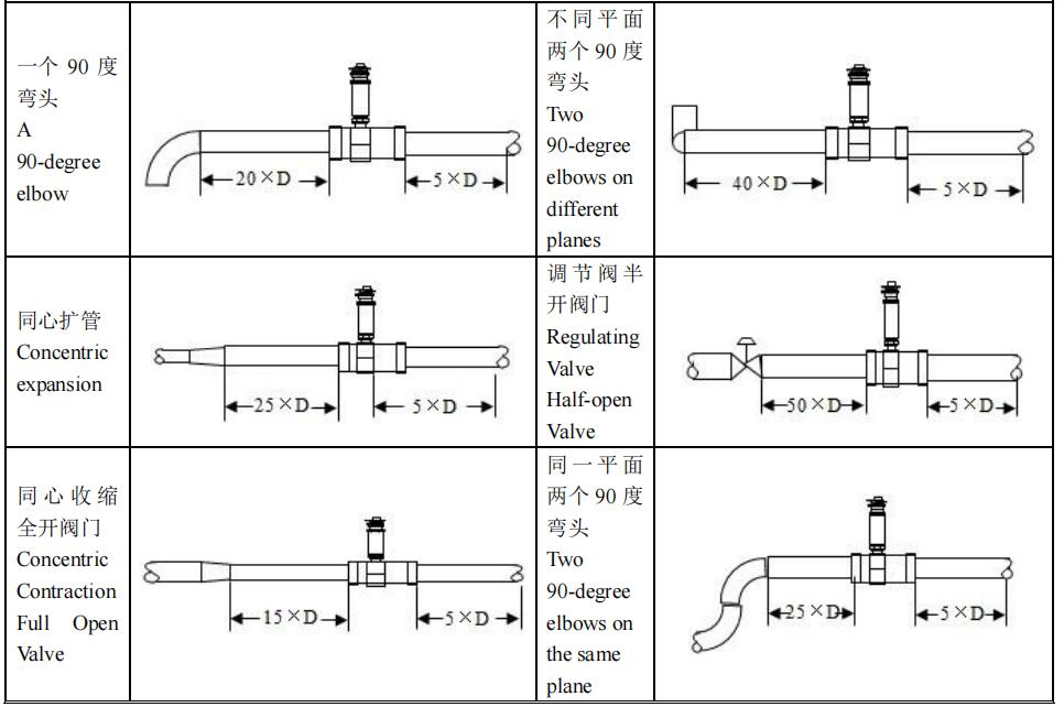
The generic field rule is 10 pipe diameters upstream and 5 downstream measured from the nearest disturbance — elbow, valve, reducer, or T. D is the internal pipe diameter. For a 2" nominal Schedule 40 pipe (ID ≈ 1.94"), that gives 19.4" before the meter and 9.7" after.

10D/5D is a starting point, not a universal truth. Magmeters tolerate 5D/3D. Vortex meters routinely need 25–35D. Coriolis meters need none. Treat 10D/5D as your default when you do not yet know the meter type — then refine against the master table below.

Why Upstream and Downstream Lengths Matter

A flow meter measures velocity (or differential pressure proportional to velocity squared). Both depend on a stable, axisymmetric velocity profile across the pipe cross-section. An elbow installed close to the meter throws a swirl into the pipe; a half-open valve creates a jet biased to one side; a reducer accelerates flow non-uniformly.

The numbers are not trivial. Field studies and the Missouri S&T flow meter piping bulletin show errors up to 50% of reading when meters sit immediately downstream of two perpendicular elbows. Straight pipe is how the disturbed profile dissipates and reverts toward fully developed flow.

The upstream length matters more than downstream because that is where the meter sees the flow. The downstream length is shorter because what comes after the sensor cannot retroactively bias the reading — it only matters because pressure recovery can propagate back upstream at low Reynolds numbers.

Straight Pipe Requirements by Meter Type

Use this as your P&ID review cheat sheet. Numbers are typical manufacturer guidance for a single elbow upstream. Two elbows in different planes can double the upstream requirement.

Meter TypeUpstreamDownstreamNotes
Orifice / DP (β = 0.5)15D5Dβ-ratio dependent; ISO 5167
Orifice / DP (β = 0.7)10D5DLower β tolerates less
Magnetic5D3DMost forgiving; keep pipe full
Vortex15–35D5D35D for two elbows in different planes
Turbine15–20D5DInclude strainer in upstream length
Ultrasonic (transit-time)10–15D5D10D for inline; 20D for clamp-on
Coriolis0D0DInsensitive to flow profile
Insertion / averaging Pitot20–50D5DProbe creates its own disturbance
Thermal mass10D5DSensitive to swirl, not profile
Variable area (rotameter)0D0DMust be vertical, flow up
Positive displacement0D0DMechanical measurement

Orifice and DP Meters: Beta Ratio Drives Length

ISO 5167-1 and ASME MFC-3M govern orifice plate installations. The required upstream length is a function of two things: the beta ratio (orifice bore / pipe ID) and the type of upstream fitting.

At β = 0.5 with a single 90° elbow upstream, ISO 5167-2 Table 3 requires 14D minimum and 28D for zero additional uncertainty. At β = 0.7, the requirement climbs to 26D minimum (and 44D for zero added uncertainty) because the contraction is sharper and disturbances bias the discharge coefficient more. Conditioning orifice plates with four-hole or perforated patterns cut this to 2–6D regardless of β.

For wedge and Venturi meters, the requirements relax — Venturi can tolerate 4–6D upstream with a single elbow. A wedge flow meter is a useful drop-in when retrofitting limited straight runs in slurry service (see our companion guide on flow meter K-factor chart).

Magnetic Flow Meters: 5D Upstream, 3D Downstream

Magnetic flow meters are the most forgiving major technology. Faraday’s law measures average velocity directly across the cross-section, so a moderately distorted profile averages out. Industry guidance is 5D upstream and 3D downstream from the electrode plane.

Two installation rules trump the straight-pipe number for magmeters. First, the pipe must remain full at the electrode plane — install in a vertical line with flow up, or in a horizontal line with the electrode axis horizontal. Second, grounding rings (or PTFE-lined grounding electrodes) carry signal noise away; missing grounding does more damage than missing straight pipe. For a deeper installation walkthrough see our magnetic flow meter installation guide.

Vortex Flow Meters: The 35D Reality

Vortex shedding requires a stable, axisymmetric inlet profile. Yokogawa’s tutorial for the YEWFLO vortex line and Cross Company’s bulletin both put the typical upstream requirement at 35 pipe diameters and downstream at 5D. That is uncomfortably long for most real plants.

Three practical relaxations: (1) some vendors allow K-factor recalibration trims for 15–20D installations; (2) a tube-bundle flow conditioner ~7D upstream cuts the requirement to 10D; (3) reducer-vortex meter designs include an integral conditioning section. For steam metering where straight runs are scarce, the reducer-vortex variant from our vortex flow meter line is the standard fix.

Turbine and Ultrasonic Meters

Turbine flow meters need 15–20D upstream with the strainer counted as part of that length. Two elbows in different planes push the requirement to 50D. Industrial turbines for custody transfer typically ship with a paired conditioner section to make the total skid 15D. Always specify a strainer with mesh ≤ 0.5 × the smallest moving-part clearance.

Ultrasonic transit-time meters measure path-averaged velocity, so they tolerate more profile distortion than vortex but less than magmeters. Inline ultrasonic spool-piece meters need 10D upstream; clamp-on retrofit installations need 20D because the transducer cannot compensate for swirl. AGA Report No. 9 governs custody-transfer ultrasonic installations for gas; API MPMS Chapter 5.8 covers liquid.

Coriolis, Rotameter, and Positive Displacement

Three technologies sidestep straight-pipe constraints entirely. Coriolis meters measure mass flow via Coriolis force on a vibrating U-tube; the measurement is insensitive to inlet profile. Rotameters use a float in a tapered vertical tube — they must be vertical with flow upward, but elbow proximity does not change the reading. Positive displacement meters trap a known volume per rotation; profile is irrelevant.

When straight pipe is truly impossible, jump to one of these three. Coriolis is the default for high-accuracy low-flow chemical injection; rotameters dominate visual local-readout duty; positive displacement remains standard for viscous fuel oil and lubricant batching.

Flow Conditioners and Plate Packs

A flow conditioner installed in the upstream run cuts the required straight pipe by 50–80% for most profile-sensitive meters. The three common types are tube bundles (4–7D long, 70% reduction), perforated plates such as the CPA 50E or NEL Mitsubishi (1D long, 60% reduction), and vane-type Etoile straighteners (3D long, 50% reduction).

Conditioners add 0.05–0.15 bar flow rate and pressure relationship drop and a procurement cost roughly 30–60% of the meter itself. They pay back when retrofitting metering into a piping run with two close elbows or when meter accuracy is more important than head loss — chemical injection skids, allocation metering, and any custody-transfer station.

ISO and ASME Standards You Can Cite

  • ISO 5167-1 through -4 — orifice plate, nozzle, Venturi installation requirements
  • ISO 6817 — electromagnetic flow meter installation
  • ISO 10790 — Coriolis installation, calibration, performance
  • ISO/TR 12764 — vortex shedding flow meter
  • ISO 2715 — turbine flow meter
  • ISO 17089 — ultrasonic gas flow meter
  • ASME MFC-3M-2004 — DP measurement of fluid flow in pipes
  • ASME MFC-11-2006 — Coriolis
  • AGA Report No. 9 — multipath ultrasonic for custody gas
  • API MPMS Chapter 5.8 — ultrasonic liquid hydrocarbon metering

5 Common Installation Mistakes

  1. Measuring upstream length from the wrong reference. The reference is the centerline of the last disturbance (elbow weld, valve seat, reducer face), not the flange. Off by one fitting and you halve the actual length.
  2. Counting strainer mesh as part of the straight pipe. A strainer creates its own disturbance. Treat it as a fitting and add 5D after it.
  3. Installing a magmeter on a horizontal line that drains partially empty. The 5D upstream is wasted if the electrodes see air at low flow. Orient the line vertical with flow up, or pump always-full.
  4. Skipping the downstream straight run because the meter is "already calibrated". Pressure-recovery effects propagate back to the sensor at low Reynolds numbers.
  5. Trusting K-factor corrections without re-proving the meter. Field correction works only if you prove against a calibrated reference in service.

FAQ

What does upstream and downstream mean in piping?

Upstream is the pipe run before the device — where the fluid is coming from. Downstream is the pipe run after the device — where the fluid is going. For a flow meter, the upstream side is the inlet face; the downstream side is the outlet.

What is 10D and 5D in flow meter installation?

10D and 5D are shorthand for "ten pipe diameters of straight pipe upstream and five downstream". D is the internal pipe diameter. The 10D/5D rule is the default starting point when meter type is unknown.

Can a flow conditioner replace straight pipe entirely?

No. A conditioner reduces the required straight length by 50–80%, but the meter still needs the conditioner to sit at least 1–7D upstream (depending on conditioner type) and 2–4D between conditioner and meter. For vortex meters, even with a tube bundle you still need 10D total.

Do Coriolis meters really need no straight pipe?

Yes — ISO 10790 confirms Coriolis meters have no upstream or downstream straight-pipe requirement for accuracy. The constraint shifts to keeping the sensor tubes full of liquid and avoiding misalignment that the meter is forced to correct.

Magnetic Water Flow Meter

DN10–DN3000 | ±0.5% | 5D/3D straight run — the most installation-forgiving full-bore meter for water, wastewater, and conductive liquids.

Vortex Flow Meter

DN15–DN300 | ±1% | Steam, gas, low-viscosity liquids. Reducer-vortex variant cuts upstream requirement to 10D.

Turbine Pulse Flow Meter

DN4–DN200 | ±0.5% | 15–20D upstream + integral strainer skid. Standard for fuel oil and clean liquid custody metering.

Need Help Picking the Right Meter for Your Piping?

Send us your line ID, fluid, flow range, and a sketch of the surrounding piping. Our process instrumentation engineers will recommend the meter technology that fits the straight pipe you actually have — and quote a complete skid if you need a conditioner.

Related: vertical pipe installation guidance.

Request a Quote

Please enable JavaScript in your browser to submit the form

Magnetic Flow Meter Installation: Straight Run, Grounding & Commissioning

A magnetic flow meter (magmeter) measures conductive liquid by Faraday’s law: when fluid moves through a magnetic field generated by the meter’s coils, electrodes pick up a voltage proportional to velocity. The physics is unforgiving — an air bubble at the electrode, an unbonded grounding ring, or a swirling pipe upstream and the meter will lie to you. Most magmeter “drift” calls in the field turn out to be installation problems, not meter problems. For meter-type selection by pipe size, accuracy, and glycol-corrected reading, see our chilled water flow meter selection by pipe size.

This guide walks the install end-to-end: required straight pipe, vertical vs horizontal mounting, flange bolt torque, grounding strategy, converter wiring, and the 10-item commissioning checklist we use on every Sino-Inst startup.

Contents

Before You Start: What You Need

  • Meter, mating flanges, gaskets, and bolts sized to the flange standard (ASME B16.5 / EN 1092-1).
  • Torque wrench (calibrated, suitable for the bolt size).
  • Grounding rings or grounding electrodes, plus #10 AWG (6 mm²) copper bonding wire.
  • Megger (insulation tester) for the post-install electrode-to-earth resistance check.
  • 4-20 mA loop checker or HART communicator for converter commissioning.
  • Confirm fluid conductivity > 5 μS/cm. Distilled water, hydrocarbons, and pure solvents do not work with magmeters.

Straight Pipe Run Requirements

Magmeters need a developed, axially symmetric velocity profile. Disturbances upstream — elbows, valves, pumps — distort that profile and shift the apparent flow rate. The accepted minima (ISO 6817 and the major OEM manuals):

The transmitter display unit — GPM, LPM, or m³/h — is software-switchable on every modern magmeter we install. If the engineering drawing is in LPM but the operator wants GPM on the local readout, set the conversion in the menu using the standard LPM to GPM factor.

Upstream DisturbanceStraight Pipe UpstreamStraight Pipe Downstream
Single 90° elbow5D3D
Two 90° elbows (in plane)10D3D
Two 90° elbows (out of plane)15D5D
Reducer / expander5D3D
Half-open valve or pump20–30D5D

D is the pipe inner diameter. If you cannot give 5D upstream, install a flow conditioner (a vaned plate or honeycomb) at the start of the straight run. We’ve seen claims that “modern magmeters don’t need straight run” — they do, just slightly less than turbines. Skipping straight run pulls the reading 2–6% off and there’s no software fix.

Vertical vs Horizontal Orientation

The first rule of magmeter mounting: the electrodes must always be wetted. The two measuring electrodes sit on opposite sides of the bore at the 3 o’clock and 9 o’clock positions when looking down the flow. Air at an electrode reads as zero conductivity and the meter goes blank.

  • Vertical pipe, upward flow: Ideal. Pipe is always full, air rises away from electrodes, sediment passes through.
  • Vertical pipe, downward flow: Acceptable only if the discharge point is below the meter so the pipe stays full. Otherwise the pipe drains and air sits at the electrodes.
  • Horizontal pipe: Rotate the meter so the electrodes are at 3 and 9 o’clock, not 12 and 6. Air pockets gather at 12; sediment settles at 6. Both kill measurement at those clock positions.
  • Avoid: mounting at the highest point of a pipeline, mounting immediately upstream of a free-discharge outlet, and mounting in a self-draining line.

Flange Bolt Torque and Tightening Sequence

Magmeter liners (PTFE, polyurethane, hard rubber, ceramic) crush easily. Over-torque and the liner deforms inward into the bore, distorting the magnetic field and changing the cross-section the fluid sees. Under-torque and the gasket leaks. Both ruin a $4,000 meter.

Always use the meter manufacturer’s torque table — values vary by liner, gasket, and flange class. As reference, typical Class 150 PTFE-lined meters call for these final torques:

Nominal SizeBolt CountFinal Torque (Class 150, PTFE)
DN50 (2″)430 N·m
DN80 (3″)450 N·m
DN100 (4″)850 N·m
DN150 (6″)875 N·m
DN200 (8″)8100 N·m
DN300 (12″)12150 N·m

Tightening sequence: snug all bolts hand-tight, then tighten in a star pattern across the flange (opposite bolts in sequence — bolt 1, 5, 3, 7, 2, 6, 4, 8 on an 8-bolt flange). Apply 30% of the final torque on the first pass, 60% on the second, 100% on the third. Re-check after 24 hours; the gasket relaxes and torque drops 10–20%.

For background on bolting and gasket selection during pressure-instrument installs, see our DP transmitter installation guide (see our companion guide on BTU meter for chilled water).

Grounding: Rings, Electrodes, and Earth Wire

The magmeter measures microvolts. The flowing liquid carries stray currents — from VFDs, cathodic protection, or simple ground-loop voltages between pumps and tanks. Without solid grounding, those currents ride on top of the Faraday signal and the reading drifts or wanders.

  • Conductive metal pipe both sides: Bond the meter housing to both upstream and downstream pipe with #10 AWG bonding wire (one strap per side, not a daisy chain). No grounding rings needed.
  • Non-conductive pipe (PVC, FRP, lined steel): Install grounding rings between the meter flanges and the pipe flanges, both sides. Bond each ring to the meter housing with #10 AWG.
  • Lined metal pipe with cathodic protection: Use grounding electrodes (a third electrode in the meter body) and connect to plant earth through the meter housing terminal. Do not bond the meter to the protected pipe.
  • Final check: Measure resistance from meter ground terminal to plant earth with a megger. Target: < 1 Ω. Anything above 10 Ω will let stray currents corrupt the reading.

Converter Mounting and Field Wiring

Compact magmeters integrate the converter on the sensor body. Remote-mount magmeters separate them — converter on a stand, sensor in the pipe — connected by a shielded multi-conductor cable. Length limits run to 30–100 m depending on coil drive voltage; do not exceed the manufacturer spec or signal degrades.

  • Mount the converter at eye level (~1.5 m), away from direct sun, vibration, and ambient above 60 °C.
  • Bring the sensor-to-converter cable in its own conduit, never sharing with VFD or motor power leads.
  • Use shielded twisted-pair cable — see our note on shielded twisted-pair cables for industrial instrumentation for the wiring details.
  • Terminate the shield at the converter end only (single-point grounding) to prevent ground-loop currents.
  • 4-20 mA output: load resistance < 600 Ω total in the loop. Use a 250 Ω resistor across the receiver input for HART communication. For analog conversion details, see our note on 4-20 mA to 0-10 V conversion.

Pre-Commissioning Checklist (10 Items)

  • 1. Flow direction arrow on meter body matches actual flow.
  • 2. Straight pipe minima met (see Section 3 table).
  • 3. Electrodes at 3 and 9 o’clock if horizontal.
  • 4. Bolt torque applied per manufacturer table, 3-pass star sequence.
  • 5. Grounding strategy executed; megger reads < 1 Ω to earth.
  • 6. Cable shield terminated at converter end only.
  • 7. Pipe pressurized and verified full (open vent until liquid escapes).
  • 8. Converter parameters set: meter size, K-factor, output scaling, damping (1–3 s typical).
  • 9. 4-20 mA loop verified end-to-end with a known input via the meter’s simulation mode.
  • 10. Zero check at no-flow with full pipe: reading should be within ±0.5% of full scale. If not, re-check grounding before calling support.

Common Installation Mistakes

  • Installing horizontally with electrodes at 12/6 o’clock. Air or sediment kills the signal. Always rotate to 3/9.
  • Skipping grounding rings in PVC piping. The meter reads but drifts unpredictably. There is no software fix.
  • Sharing conduit with VFD output cable. The PWM noise couples into the electrode signal. Use separate conduits or 300 mm spacing.
  • Over-torquing bolts to “make sure it doesn’t leak.” Crushes the liner, distorts the bore, voids the warranty.
  • Mounting upstream of a regulating valve. Cavitation on the valve opening seeds bubbles that travel back through the meter.

For installation principles that apply to most flow meter families — including turbines and Coriolis — see our turbine flow meter installation guidelines and vertical flow meter installation do’s and don’ts by meter type.

Featured Magnetic Flow Meters from Sino-Inst

Industrial Magmeter Flow Meter

DN15 to DN3000 | ±0.5% accuracy | PTFE / rubber / polyurethane liners — water, wastewater, slurry, and acid lines.
Insertion Magmeter SI-3121

Hot-tap insertion | DN80 to DN3000 | No process shutdown — for large pipes where a full-bore meter is impractical.

Stainless Steel Magmeter

SS304/SS316 body | Sanitary or industrial flange | CIP/SIP capable — food, beverage, pharma, and aggressive chemicals.

Send your pipe size, fluid, flow range, and process temperature/pressure to our engineers via the form below — we typically reply within one working day with a sized quote.

FAQ

How much straight pipe does a magnetic flow meter need?

For a single 90° elbow: 5 pipe diameters (5D) upstream and 3D downstream. Two elbows out-of-plane: 15D upstream. Valves and pumps: 20–30D upstream. Skipping straight run pulls accuracy 2–6% off, and no software fix exists.

Can a magnetic flow meter be installed vertically?

Yes — vertical with upward flow is the ideal mounting because the pipe stays full, air rises away from electrodes, and sediment passes through. Vertical with downward flow only works if the pipe stays full downstream of the meter.

Do I need grounding rings for a magnetic flow meter?

Grounding rings are required when the upstream or downstream pipe is non-conductive (PVC, FRP, lined steel) — one ring on each side. For continuous conductive metal pipe both sides, a simple bonding wire from meter housing to each pipe section is enough.

What is the minimum conductivity for a magnetic flow meter?

Most magmeters need 5 μS/cm minimum. A few high-impedance designs work down to 1 μS/cm. Magmeters do not work on hydrocarbons, distilled water, or non-polar solvents — use Coriolis or ultrasonic for those.

What flange bolt torque do I use on a magnetic flow meter?

Always follow the meter manufacturer’s torque table — values depend on liner material and gasket. As reference, Class 150 PTFE-lined meters call for 30 N·m at DN50 up to 150 N·m at DN300. Apply in three passes (30/60/100%) using a star pattern, then re-check after 24 hours.

Can I install a magnetic flow meter near a pump?

Always downstream, never upstream — pumps generate swirl that an upstream meter cannot resolve. Allow 20–30D of straight pipe between pump discharge and meter inlet. If space is tight, install a flow conditioner at the start of the run.

Request a Quote

Please enable JavaScript in your browser to submit the form

Related: straight-pipe requirements for flow meter installation.

What Is a Flow Transmitter? Working Principle, Signal Output, and How It Differs from a Flow Meter

Updated 2026-05-09 by the Sino-Inst engineering team.

A flow transmitter is the field instrument that turns a flow measurement into a 4-20 mA, HART, Modbus, or pulse signal that a PLC or DCS can read — and that a SCADA historian then trends across the plant. It sits between a primary element (an orifice plate, a magmeter coil, a vortex bluff body, a Coriolis tube) and the control room. This guide explains what is inside a flow transmitter, how each signal output works, how the device differs from a plain flow meter, and the five spec-sheet numbers that decide whether a transmitter actually fits the loop.

Contents

The Role of a Flow Transmitter in a Process Loop

Picture a typical 4-20 mA loop in a chemical plant. A primary element — say, an orifice plate — sits in the line and produces a measurable physical effect (a pressure drop). A flow transmitter reads that effect, applies the calibration curve, and outputs a single proportional signal: 4 mA at zero flow, 20 mA at full scale. The control room receives that one wire pair and treats it as the flow value.

That is the practical definition. A flow transmitter is the part that does three jobs: it senses, it conditions, and it transmits. A bare flow sensor cannot drive a 1500-foot cable run to a marshalling cabinet. A 4-20 mA transmitter can, because the signal is a current, not a voltage, and is immune to wiring resistance up to the loop budget.

For a deeper view of how the loop carries the signal, see our guide on upstream and downstream straight pipe requirements, which covers the install conditions that decide whether the reading you transmit is even valid.

Inside a Flow Transmitter: Primary Element, Sensor, Transducer, and Output Stage

A complete flow-measurement chain has four stages. Each stage has a job, and changing one without considering the others is the most common reason a “calibrated” loop reads the wrong number.

  1. Primary element — the device in the pipe that creates a measurable effect. Orifice plate, venturi tube, magmeter electrodes, vortex bluff body, Coriolis tube, ultrasonic transducers. Each has its own physics.
  2. Sensor — the part that reads the effect. A differential-pressure cell across an orifice. Two electrodes across a magmeter. A piezoelectric crystal behind a vortex bluff body. The sensor outputs a small electrical quantity (millivolts, microamps, picocoulombs).
  3. Transducer / signal conditioner — the analog and digital electronics that linearise, temperature-compensate, and scale the sensor signal into engineering units. This is where the calibration curve lives.
  4. Output stage — the transmitter proper. Drives 4-20 mA, encodes HART on top, talks Modbus RTU/TCP, or generates a scaled pulse output.

Take a magnetic flow transmitter as a worked example. The coils generate field B inside the meter body. Conductive liquid passing through cuts the field at velocity v, and Faraday’s law gives an induced EMF: V = k · B · D · v, where D is the bore diameter. That induced voltage is in the millivolt range. The transducer amplifies it, removes 50/60 Hz noise, applies the calibration K-factor, and the output stage scales the result to a 4-20 mA current loop.

Signal Output Options: 4-20 mA, HART, Modbus, and Pulse

The output you pick is dictated by what the receiving system speaks. Most modern transmitters offer two or more options on the same hardware, but mixing them is non-trivial.

OutputTypical useWiringPractical limit
4-20 mA analogContinuous flow rate to PLC/DCS analog inputTwin shielded, up to ~1500 m at 24 V loopOne value per pair; ~0.05% reading resolution at ADC
HART (over 4-20 mA)Diagnostics + secondary variables on existing 4-20 mA wiringSame twin shielded; HART superimposes 1200 baud FSKSlow data rate; needs HART-aware host
Modbus RTU/TCPMultivariable digital data — flow + totalizer + diagnosticsRS-485 multidrop (RTU) or Ethernet (TCP)Up to 247 nodes per RS-485 segment
Pulse / frequencyTotalizing into a counter (custody transfer, batching)Open collector or scaled frequencyOne pulse = one volume unit; needs care for low flow rates

For batch control or custody transfer, pulse output is still the most defensible because the count is unambiguous. For instrumentation under modern asset-management software, HART is the path of least resistance — every modern handheld speaks it. See our note on converting a 4-20 mA loop to 0-10 V when the receiver is a legacy voltage input.

How a Flow Transmitter Differs from a Flow Meter

The two terms get used loosely. Strictly, a flow meter is a device that indicates flow rate locally — a rotameter with a glass tube and a float, a paddlewheel with a mechanical totalizer, a magmeter with a field LCD. A flow transmitter is the version that also outputs a remote signal. Many modern devices integrate both: a magmeter body with a digital display on the converter, plus 4-20 mA / HART / Modbus to the control room. The same hardware sells under either name depending on whether the brochure is aimed at a maintenance engineer or a control engineer.

The practical decision is not about the names. It is about whether the value needs to leave the field, and over which protocol. If you only need a local read for plant rounds, a basic flow meter is enough. If a PLC or DCS must log the value, alarm on it, or use it in a control loop, a transmitter is required. See flow totalizer vs flow meter for the related distinction between rate-only and totalising units.

Reading a Flow Transmitter Spec Sheet — Five Numbers That Matter

A spec sheet is a contract. Five numbers do most of the work; the rest is decoration.

  • Calibrated range and turndown — the ratio between the highest and lowest flow the device measures within accuracy. A magmeter at 100:1 turndown is honest from 0.3 m/s to 30 m/s. A DP transmitter at 10:1 is fine in a steady-state line, painful in a varying batch process.
  • Accuracy class — read whether it is “% of reading” or “% of span”. 0.5% of reading at 10% of span is 5x worse than 0.5% of full scale near zero. Vendors quote whichever number looks better.
  • Process and ambient temperature — separate ratings. The wetted body sees process fluid temperature; the electronics housing sees ambient. The lower of the two limits is the one that bites.
  • Output and protocols — confirm 4-20 mA loop voltage budget (typically 12-42 V), HART revision, and Modbus addressing. Do not assume; ask.
  • Hazardous-area certification — ATEX, IECEx, FM/CSA, and the gas/dust group. A transmitter rated Zone 2 will not be accepted by the safety case for a Zone 0 vessel headspace.

For installation context that affects what numbers you actually achieve in the field, see our differential pressure flow meter calculation guide and the flow units cheat sheet when reading a US-units brochure.

Industrial Magmeter Flow Meters

Conductive liquids, DN10–DN3000. 4-20 mA + HART, accuracy ±0.5% of reading, IP68 sub-DN200.

Vortex Shedding Flow Meter

Steam, gas, low-viscosity liquid. 4-20 mA / HART / pulse. Up to 426 °C process temp, no moving parts.

Wedge Flow Meter

Slurries, dirty / abrasive fluids. DP-based, 4-20 mA / HART, recoverable signal at low Reynolds number.

Flow Transmitter FAQ

How does a flow transmitter work?

A flow transmitter reads a primary element (orifice, magmeter, vortex, Coriolis) through a sensor, applies the calibration in a transducer, and outputs a 4-20 mA, HART, Modbus, or pulse signal proportional to flow rate.

What is the difference between a pressure transmitter and a flow transmitter?

A pressure transmitter outputs a signal proportional to gauge, absolute, or differential pressure. For fast dynamic events such as engine in-cylinder combustion or hydraulic pulsations, a piezoelectric pressure sensor is used instead. A flow transmitter outputs a signal proportional to flow rate. A DP-based flow transmitter combines a DP cell with a primary element and a square-root extraction stage.

What are the three types of transmitters used in flow measurement?

Differential-pressure (orifice, venturi, wedge), velocity (magmeter, vortex, ultrasonic, turbine), and mass-flow (Coriolis, thermal).

What is the purpose of a flow transmitter in a process loop?

To convert a measured flow into a control-room-readable signal that can be logged, alarmed, used in a PID loop, or fed into custody transfer at any distance from the field.

Get a Quote from Our Flow Engineering Team

Tell us your line size, fluid, expected flow range, and required output protocol. Our engineers will respond within one business day with a recommended transmitter, datasheet, and lead time.

Request a Quote

Please enable JavaScript in your browser to submit the form

Related: flow rate unit conversions.

Refrigerant Flow Meter: Coriolis, Vortex, Ultrasonic by Refrigerant Type

A refrigerant flow meter must do something a water flow meter does not: handle a fluid whose density swings from 30 kg/m³ in the suction line to over 1300 kg/m³ in the liquid line of the same chiller. That density swing is why mass-flow Coriolis dominates the high-accuracy refrigerant market, why thermal-mass meters fall over on phase change, and why magnetic flow meters are simply wrong for any refrigerant — none of the common HFC, HFO, hydrocarbon, or natural refrigerants conducts electricity. This guide matches meter technology to refrigerant by chemistry and phase, names the install rules that protect the reading, and gives the buyer numbers that decide between a $3 k vortex and a $14 k Coriolis. For meter-type selection by pipe size, accuracy class, and glycol correction, see our chilled water flow meter selection guide.

Contents

Why Refrigerant Flow Is Not Water Flow

Refrigerant flow measurement breaks three assumptions that make water flow easy. First, density is a strong function of pressure and subcooling — R134a liquid at 5 °C / 350 kPa is 1295 kg/m³, but at 50 °C / 1320 kPa it drops to 1102 kg/m³, a 15% swing on a single charge cycle. Second, two-phase flow is normal: an ill-installed orifice meter sees flashing past the vena contracta and reads chaotic noise. Third, the fluid is non-conductive, ruling out the magmeter that would otherwise be the cheapest answer.

The practical consequence: any volumetric meter (vortex, turbine, ultrasonic, oval-gear) requires a corrected density input to deliver mass flow, which is what the refrigeration cycle calculation actually needs. Coriolis short-circuits this by measuring mass flow directly through the inertial deflection of an oscillating tube, independent of density and viscosity. That is why every chiller-OEM commissioning skid we have inspected uses Coriolis, even when the project budget pretends otherwise.

Match Refrigerant Type to Meter Technology

Refrigerant family decides the candidate technologies before flow rate or pipe size. Hydrocarbon refrigerants (R290 propane, R600a isobutane) demand intrinsically safe construction because charges above 150 g cross the IEC 60335-2-89 flammable threshold. CO2 (R744) at 70–110 bar in transcritical mode pushes mechanical meters off the spec sheet entirely. Ammonia (R717) corrodes copper, so any meter with brazed Cu-tube wetted parts is out.

RefrigerantClassTypical pressureBest meterAvoid
R134a, R513AHFC / HFO blend2–15 barCoriolis (liquid line); vortex (vapor)Magmeter (non-conductive)
R410A, R32HFC10–35 barCoriolis (subcooled liquid)Turbine in two-phase service
R290, R600a, R1270Hydrocarbon (A3)4–20 barCoriolis with ATEX Ex iaAny non-IS sensor
R744 (CO2)Natural40–110 bar transcriticalCoriolis rated 150–200 barVortex below transcritical pinch
R717 (NH3)Natural6–18 barCoriolis 316L SS; vortex SSAny copper-bearing wetted part
R1234yf, R1234zeHFO3–9 barCoriolis with low-flow tubeOrifice (high pressure-loss)

One rule survives across all six rows: pick a meter whose pressure rating is at least 1.5 × the relief-valve setpoint of the system. CO2 transcritical service routinely rejects meters specified at 50 bar — the gas cooler outlet sits at 95 bar at 35 °C ambient, and 110 bar in summer.

Coriolis Mass Flow: When the Spec Demands Mass Accuracy

Coriolis is the default refrigerant flow meter for any application where mass accuracy decides the outcome — refrigerant charging skids, OEM performance test stands, energy-audit submetering, leak-detection mass balances, and any custody-transfer point in industrial NH3 or CO2 service. Accuracy of 0.1–0.2% of mass flow rate is achievable down to 1% of full-scale turndown.

  • Mass directly, no density correction. The oscillating-tube principle reads kg/h regardless of subcooling or pressure shift, so a single calibration covers the full operating envelope.
  • Built-in density measurement. Many Coriolis transmitters output fluid density (g/cm³) as a second 4–20 mA channel — useful for confirming refrigerant condition or detecting oil entrainment in the liquid line.
  • Bidirectional flow. The same meter handles charge and recovery cycles without re-zeroing, valuable on heat-pump four-way valve systems.
  • Wide turndown. 100:1 turndown means one meter sizes for both winter and summer load profiles on a single chiller.

The downsides are cost (a 1″ Coriolis transmitter is typically 5–8× the price of a vortex of the same line size), pressure drop (especially on small-flow models with the U-tube geometry — see our guide on viscous-fluid flow meters for the same trade-off discussion), and sensitivity to mounting vibration on packaged compressor skids. For low-flow refrigerant service (under 50 kg/h, typical of mini-split test stands), the T-series triangle Coriolis geometry beats the standard U-tube on accuracy at the bottom of the range.

Vortex and Ultrasonic Meters: Lower-Cost Volumetric Options

When the application is vapor-line metering — discharge line flow on a chiller, suction-line flow on a refrigeration rack — vortex shedding is the price-performance sweet spot. A vortex meter measures volumetric flow rate, which the DCS converts to mass using a temperature-compensated density polynomial for the refrigerant in question. Accuracy of 1.0% of rate is typical; turndown 20:1 on gas service.

TechnologyAccuracyTurndownBest phaseIndicative price (1″ DN25)
Coriolis (mass)0.1–0.2% rate100:1Liquid; gas with care$8 k–$14 k
Vortex (volumetric)1.0% rate20:1Vapor / superheated gas$2 k–$3.5 k
Ultrasonic (volumetric)1.0–2.0% rate50:1Subcooled liquid only$3 k–$5 k
Turbine (volumetric)0.5% rate10:1Single-phase liquid$1.5 k–$3 k
Thermal mass2–3% rate50:1Pure single-phase gas only$2.5 k–$4.5 k

Ultrasonic transit-time meters work on subcooled liquid refrigerant lines if the line is full and free of vapor bubbles. They struggle in two-phase service. Thermal mass meters give acceptable accuracy on dry vapor only — any liquid carryover destroys the calibration because liquid latent heat distorts the thermal-dispersion equation. For natural-gas lines on absorption chillers (LiBr/H2O machines using natural gas as fuel) the picture differs — see our straight-pipe requirements guide for the install-length rules that govern vortex and ultrasonic accuracy on gas service.

Liquid Line vs. Vapor Line: Phase Decides the Meter

The single rule we apply on every refrigerant flow project: identify the phase at the meter location first; pick the technology second. A meter sized for liquid that occasionally sees flash gas will mis-read by 30% during the flash event, then reset normally. A meter sized for superheated vapor that occasionally sees liquid carryover will deliver an accuracy band the customer never specified.

  • Liquid line, post-condenser, subcooled ≥ 5 K. Coriolis or ultrasonic. Confirm subcooling at the meter — if the line runs uphill or through a low spot, install the meter at the low spot to keep the line full.
  • Liquid line, post-receiver, sight-glass clear. Coriolis preferred. Turbine acceptable for single-charge custody transfer.
  • Discharge vapor, post-compressor, superheated 10–40 K. Vortex for low-cost; Coriolis if the spec calls for ±0.5%.
  • Suction vapor, low pressure, 5–20 K superheat. Vortex sized for the lowest density point; thermal mass only if liquid floodback is excluded by upstream protection.
  • Two-phase line, expansion valve outlet to evaporator inlet. No meter type works reliably here. Move the measurement upstream to single-phase liquid or downstream to single-phase vapor.

Plant Types: Chiller, VRF, Supermarket Rack, Industrial NH3

Where the meter sits on the plant influences both the chosen technology and the certification requirement. Four common installations recur in our project files.

  • Centrifugal water chiller (HFC / HFO): Coriolis on liquid line post-condenser for performance test, vortex on hot-gas bypass when present. Typical line size DN50–DN100.
  • VRF / VRV (R410A, R32): Coriolis at the outdoor-unit liquid header for energy submetering by zone. Compact Z-series straight-tube preferred to keep packaging within rooftop dimensions.
  • Supermarket CO2 rack (R744): Coriolis rated 150–200 bar on liquid receiver outlet for charge accountability; vortex on flash-gas bypass to MT/LT loads.
  • Industrial NH3 (R717) cold storage: Coriolis 316L SS on king-valve liquid line; vortex SS on hot-gas defrost line; no copper-wetted parts. Pair with our ammonia flow meter selection guide for full ammonia-system specification rules.

Featured Refrigerant Flow Meters

Z-Series Straight-Tube Coriolis Flow Meter

Compact straight-tube Coriolis for liquid-line refrigerant on chiller and VRF systems. 0.1% mass accuracy, 200 bar option for CO2 transcritical service, ATEX Ex ia for hydrocarbon refrigerants.

T-Series Triangle Coriolis Mass Flowmeter

Low-flow triangle-tube geometry for refrigerant charging skids and OEM mini-split test stands. Maintains 0.2% accuracy at 1 kg/h on R290, R134a, and R1234yf charging duties.

Split High-Temperature Vortex Flow Meter

Lower-cost volumetric option for discharge-line vapor metering up to 250 °C. Split design isolates the transmitter electronics from compressor-skid heat. ±1% rate, 20:1 turndown.

FAQ

Can I use a magnetic flow meter for refrigerant?

No. Magnetic flow meters need an electrolyte conductivity above 5 µS/cm; common refrigerants (HFC, HFO, hydrocarbons, CO2) are non-conductive and produce no electromotive force across the magnetic field. The meter will read zero or noise. Use Coriolis for mass-accurate refrigerant flow.

What is the most accurate refrigerant flow meter?

Coriolis mass flow meters reach 0.1% of mass flow rate on subcooled liquid refrigerant — about an order of magnitude better than vortex or ultrasonic. The accuracy holds across the full pressure and temperature range because the principle measures inertial force, not volume.

Will a Coriolis meter work on R744 (CO2) at transcritical pressures?

Yes, but only with a specifically rated body. Standard 100 bar Coriolis bodies are not safe at the 95–110 bar gas-cooler outlet pressures common in summer. Specify a 150–200 bar wetted-part rating for transcritical CO2 service, with NACE MR0175-compliant wetted parts when sour-gas trace is suspected.

Why does my vortex meter read poorly on a refrigeration suction line?

Two reasons usually combine. First, suction-line vapor density at low evaporator temperature drops below the vortex meter’s minimum Reynolds number, putting the operating point in the dropout zone. Second, liquid floodback from the evaporator (transient or chronic) lands as droplets on the bluff body and produces noise. Move the meter to the discharge line, or upsize the suction line to keep velocity in band.

Do I need an ATEX-rated meter for R290 propane?

If the system charge exceeds the IEC 60335-2-89 limit (typically 150 g for self-contained equipment, higher for split systems with leak-detection), yes. Specify Coriolis or vortex with ATEX Ex ia (intrinsically safe) certification, plus a Zener barrier or galvanic isolator at the safe-side panel. Below the charge limit the equipment is exempt, but most building-services projects still require IS construction by site policy.

Can ultrasonic flow meters measure refrigerant?

Transit-time ultrasonic meters work on subcooled, single-phase liquid refrigerant in a full pipe. They do not handle two-phase service or vapor lines reliably because acoustic propagation through bubbly or low-density media is unstable. For a chilled-water side of an absorption chiller the picture is different — see our BTU meter for chilled water guide for that case.

For a refrigerant-specific quote — chemistry, line size, pressure, and target accuracy — our application engineers respond within one working day with a sized Coriolis or vortex configuration, including ATEX certification path and pressure drop calculation.

Request a Quote

Please enable JavaScript in your browser to submit the form

How Does a Piston Flow Meter Work? Cycle, Specs & PD Comparison

A piston flow meter measures liquid by counting how many fixed-volume slugs pass through the meter body. Each rotation of the piston pushes one chamber of liquid past a sealed reference, and a magnet on the piston shaft drives a register or a pulse output. Because the volume per cycle is mechanical — set by the bore and stroke at the factory — a piston meter is one of the most accurate ways to measure low-flow viscous liquids without depending on electronics inside the wet path.

PD meters generate one pulse per displacement cycle — the pulse count per litre is the meter’s K-factor, and it is stamped on the calibration certificate.

Contents

A Piston Flow Meter in One Sentence

A piston flow meter is a positive-displacement (PD) flow meter in which a piston sweeps a fixed volume of liquid through a precision-bored cylinder once per cycle, and a magnet-coupled counter totalises cycles into volume. Because the volume per cycle is fixed by hardware, accuracy is independent of fluid viscosity, conductivity, or temperature within the meter’s operating window — a property no inferential meter (turbine, magnetic, ultrasonic) can match.

The same physics that makes piston meters accurate also makes them the best fit for very low flow (down to a few mL/min) and high-viscosity service (up to ~10,000 cP). Below we walk through the cycle, the two common geometries, and where the piston wins versus the gear, oval-gear, and nutating-disc PD meters.

The Four Phases of One Piston Cycle

One full piston cycle moves a known volume — the swept volume of the cylinder — from inlet to outlet. The cycle is mechanically forced by the inlet pressure; there is no motor and no electronic actuation in the wet path.

  1. Inlet fill. Inlet pressure forces liquid into chamber A on the inlet side of the piston. The piston is at one end of its stroke, and chamber B (on the outlet side) is full.
  2. Crossover. A slide valve or rotary valve, mechanically linked to the piston, switches the inlet port from chamber A to chamber B and the outlet port from chamber B to chamber A.
  3. Discharge / fill. Now chamber B fills while chamber A discharges through the outlet. The piston moves to the opposite end of the stroke.
  4. Pulse and reset. A magnet on the piston shaft passes a Hall sensor or reed switch, generating one pulse per cycle (or per half-cycle, depending on geometry). The valve crossover happens again, and the next cycle begins.

Volume per pulse is set by the cylinder bore and stroke: Vpulse = π × (D/2)² × L, factory-calibrated and stamped on the meter nameplate. Typical pulse volumes range from 0.5 mL/pulse on a micro-flow meter up to 1 L/pulse on a large oil meter.

Oscillating Piston vs. Reciprocating Piston

Two piston geometries share the “piston flow meter” label, and they have different performance envelopes.

  • Reciprocating piston. The piston moves linearly in a cylinder. A crank or slide valve switches the ports at each end of the stroke. Used for very low flow and high precision (volumetric uncertainty <0.1% of reading achievable). The piston is single-acting (one chamber) or double-acting (two chambers, one cycle counts twice).
  • Oscillating (rotary) piston. A hollow ring-shaped piston oscillates around a central partition inside a cylindrical chamber. There is no separate valve — the piston geometry itself ports the inlet and outlet flows. Each oscillation displaces a fixed annular volume. Cheaper to build, more tolerant of dirty fluids, slightly lower accuracy (typically ±0.5% of reading).

Reciprocating piston meters dominate laboratory and chemical-injection service where 0.1% accuracy is required. Oscillating piston meters dominate utility water sub-metering and small-batch chemical dosing where 0.5% is acceptable and the lower cost wins.

Accuracy, Turndown, and Viscosity Window

Three numbers define whether a piston meter fits an application: accuracy, turndown, and the viscosity window over which the accuracy holds.

SpecReciprocating pistonOscillating pistonWhy it matters
Accuracy±0.05% to ±0.2% of reading±0.5% to ±1.0% of readingCustody transfer needs ≤0.2%
Repeatability±0.02%±0.05%Critical for dosing
Turndown50:1 typical, 100:1 in lab10:1 to 20:1Wide-range process flow
Min flow0.5 mL/min50 mL/minCatalyst/additive injection
Max flow50 L/min500 L/minBulk fuel transfer
Viscosity0.5–10,000 cP (hot oil 50,000+ cP)0.5–500 cPHeavy fuel, polymer, syrup
Pressure drop @ rated flow0.3–1 bar0.1–0.3 barLow-head systems

The viscosity window is the most underappreciated spec. Inferential meters (turbine, magnetic, vortex) lose accuracy as viscosity rises because the velocity profile inside the meter changes. A piston meter does not — the swept volume is the swept volume regardless of how slowly the liquid moves through it. That is why piston (and other PD) meters are the default for fuel oil, asphalt, and polymer dosing.

Piston vs. Other Positive-Displacement Meters

Piston is one of four common PD geometries. The choice between them is rarely “which is most accurate” — they’re all accurate by design — but rather which geometry fits the fluid, the flow range, and the maintenance budget.

PD geometryAccuracyBest fluidParticle toleranceNotes
Piston (reciprocating)±0.05–0.2%Clean low-viscosity to thick polymerLow (≤25 µm)Highest accuracy of the PD family
Piston (oscillating)±0.5–1%Water, fuel, oilsMedium (≤100 µm)Cheaper, looser tolerance
Oval gear±0.2–0.5%Viscous oils, diesel, lubeLow (≤50 µm)Good for high-viscosity custody transfer
Helical gear±0.2–0.5%High-viscosity, high-flowLow (≤50 µm)Lower pressure drop than oval at same flow
Nutating disc±1.0–1.5%Cold water, building serviceMediumThe “domestic water meter” geometry
Rotary lobe±0.3%Food, dairy, viscous chemicalsMediumSanitary clamp body; CIP-cleanable

The decision rule we use:

  • Need ≤0.1% accuracy on a clean low-flow stream → reciprocating piston.
  • Need 0.2–0.5% on viscous oil at moderate flow → oval gear or helical gear.
  • Sub-metering water or simple fuel transfer with ±1% acceptable → oscillating piston or nutating disc, whichever is on the shelf.
  • Sanitary food/dairy or polymer dosing in a CIP loop → rotary lobe.

For a side-by-side on the gear vs piston decision specifically, see our turbine vs gear flow meter comparison; both gear families share most of their decision logic with the piston meter.

Where the Piston Geometry Wins

Three application classes consistently push the spec line to a piston flow meter rather than another PD or an inferential meter.

  • Chemical injection and additive dosing. Catalyst, biocide, scale inhibitor, dye into a process line at flows of 1–500 mL/min. The 50:1 turndown of a reciprocating piston covers the full operating envelope of one injection skid.
  • Fuel and lubrication oil custody transfer at low flow. Burner pump skids, generator day-tank metering, lube-oil dispensing carts. Viscosities of 5–500 cP at moderate temperature; piston accuracy holds where a turbine would slow and slip.
  • Laboratory and pilot-plant flow measurement. Reactor feed streams, micro-distillation, polymer process development. The volume-per-cycle calibration travels with the meter, no flow standard needed in the lab.

For high-viscosity oil service specifically, see our oval-gear high-viscosity flow meter notes — at viscosities above 1000 cP the gear geometry sometimes beats the piston on pressure drop.

Installation Rules and Failure Modes

Piston meters are mechanically simple but unforgiving on installation. Three install errors account for the bulk of warranty returns.

  • Strainer upstream is mandatory. 25 µm cartridge for reciprocating, 100 µm Y-strainer for oscillating. A single grit particle in the cylinder gap scores the bore; once scored, the volumetric reference is gone and the meter is scrap. This is the single biggest reason piston meters fail in service.
  • Vapor lock and entrained air. Any air in the inlet pulses the piston at the air’s effective volume — usually higher than the liquid — causing positive bias. Mount horizontally, with a vent or an upstream air separator if the line is gravity-fed or has a pump suction issue.
  • Pressure surge on start-up. A check valve closing into a piston meter creates a hammer that can fracture the cylinder casting. Add a soft-start sequence on the upstream pump, or a dampener on the line.

Most reciprocating piston meters also need an annual recalibration check. The wear is at the piston-to-bore clearance — <25 µm new, sometimes 50 µm after a year of service — which slips a small but measurable percentage of liquid past the piston without counting it. Recalibrate against a master meter or a gravimetric stand and re-stamp the K-factor on the nameplate.

Featured Positive-Displacement Flow Meters

The three meters below cover the three roles a piston-class meter is typically asked to fill — pure mechanical pointer for non-electrical service, electronic helical-gear PD for high-viscosity custody transfer, and sanitary clamp-mount PD for food/dairy dosing.

Pointer-Type Oval Gear Flow Meter

All-mechanical PD meter for non-electrical service: diesel transfer, hydraulic fluid, gear oil. Local pointer + 8-digit totalizer, no power needed. ±0.5% accuracy, viscosity 2–200 cP, DN15–DN100 sizes.

Helical Gear PD Flow Meter

Electronic PD meter for high-viscosity custody transfer: heavy fuel oil, lube oil, polymer melt to 10,000 cP. Pulse + 4–20 mA + Modbus output, ±0.2% accuracy. Lower pressure drop than oval-gear at the same flow.

Sanitary Tri-Clamp PD Flow Meter

Sanitary clamp-mount PD meter for food, dairy, and personal-care dosing. 316L wetted parts, EPDM seals, CIP-compatible. ±0.5% accuracy on syrups, sauces, and cosmetic emulsions to 5,000 cP.

FAQ

How does a piston flow meter measure flow?

By counting fixed-volume cycles. Inlet pressure pushes liquid into one chamber, the piston shifts, and a slide valve crossports inlet and outlet so the next chamber fills. Each piston cycle moves a precisely-known volume from inlet to outlet. A magnet on the piston shaft generates a pulse per cycle, totalised by the register or downstream PLC.

Is a piston flow meter the same as a positive-displacement meter?

Piston is one geometry of positive-displacement meter; the others are oval gear, helical gear, nutating disc, and rotary lobe. All PD meters work by trapping known volumes between mechanical surfaces and counting them, but the surface geometry differs and the application fit differs with it.

What accuracy can I expect from a piston flow meter?

±0.05% to ±0.2% of reading for a reciprocating piston in clean service; ±0.5% to ±1.0% for an oscillating piston in utility-water or simple fuel-transfer service. Repeatability is typically a factor of 10 better than accuracy, so piston meters dose chemicals more precisely than they totalise volume on a single fill.

What viscosities can a piston flow meter handle?

Reciprocating piston meters handle 0.5–10,000 cP without recalibration, with hot-oil versions extending to 50,000 cP. Oscillating piston is limited to about 500 cP. Above 10,000 cP a helical-gear PD geometry usually wins on pressure drop.

Why does my piston flow meter need a strainer upstream?

The accuracy of a piston meter depends on a precision-bored cylinder with <25 µm clearance to the piston. A single hard particle in that gap scores the bore; once scored, liquid leaks past the piston without being counted, and the meter is no longer accurate. A 25 µm cartridge or 100 µm Y-strainer immediately upstream prevents this and is a non-negotiable install requirement.

How is a piston flow meter calibrated in the field?

By comparing meter output against a master meter or a gravimetric calibration stand at three flow points (low, mid, high). The K-factor (pulses per litre or per gallon) is adjusted in the totalizer or PLC and re-stamped on the nameplate. For custody transfer the calibration certificate is renewed every 12 months; for general process service every 24 months is typical.

When should I choose a different PD meter over a piston?

Choose oval gear or helical gear when the application is high-viscosity oil custody transfer at moderate flow (the gear geometry has lower pressure drop). Choose nutating disc for cold-water sub-metering where ±1% is fine. Choose rotary lobe for sanitary food/dairy/cosmetic dosing where the meter has to be CIP-cleanable. Stay with piston when accuracy must be ≤0.2% on low flow or the turndown must exceed 30:1.

If you’re sizing a meter for a chemical injection skid, a fuel custody transfer point, or a low-flow viscous service, send the fluid type, viscosity at operating temperature, flow range, and required accuracy — our team will reply with two or three meter options and the K-factor analysis within one business day.

Request a Quote

Please enable JavaScript in your browser to submit the form

Solid Flow Meter: 6 Technologies Compared, Decision Matrix by Material

A solid flow meter measures the mass flow of dry bulk material — cement, soybean meal, fly ash, plastic pellets, sugar, mined coal — moving through a pipe, chute, or on a belt. Unlike liquid flow, there is no single dominant technology: impact-plate, microwave Doppler, Coriolis, belt-weigher (LIW), and nucleonic meters all have their place, and picking the wrong one will cost you 20–30 % accuracy on a tonne-per-hour basis.

This guide is built around a six-technology comparison and a material-driven decision matrix. Use it to narrow down to one or two candidates before pricing — most procurement mistakes we see come from sizing a microwave meter for a slow gravity chute, or specifying an impact plate for an abrasive that destroys plates in three months.

Contents

What Counts as a “Solid Flow”

A solid flow is a dry, particulate stream where the material is conveyed by gravity, mechanical (screw, belt, drag-chain), or pneumatic (dilute or dense phase) means. Particle size ranges from sub-µm fly ash up to 50 mm coal lumps, bulk densities from 50 kg/m³ for puffed rice to 2400 kg/m³ for iron ore, and flow rates from a few kg/h on a feeder weigher to 5000 t/h on a coal handling belt.

Two physical realities drive the technology choice:

  • Velocity profile. Pneumatic-conveyed solids move at 15–25 m/s; gravity-fed solids in a chute fall at √(2gh)≈3–6 m/s; on a belt they move at 1–3 m/s. Each speed range favours different sensor physics.
  • Density variability. Bulk density of the same material can vary ±10 % with moisture, packing, and aeration. Volumetric meters (microwave, ultrasonic) can not correct for this; mass-based meters (impact plate, Coriolis, belt scale) can.

Six Technologies Compared

Six measurement principles cover almost every solid flow application. Pick by conveying mode first, then by material abrasiveness, then by accuracy class.

TechnologyPrincipleConveying modeTypical accuracyRangeSweet spot
Impact plateForce on a deflector plateGravity chute±0.5–1 % FS1–500 t/hCement, grain, sugar
Microwave DopplerReflected frequency shiftPneumatic / gravity±2–5 % FS0.05–200 t/hFly ash, dust, fine powder
Coriolis (mass)Coriolis force on rotating measuring wheelFree-falling stream±0.5 % FS0.1–600 t/hFree-flowing granules, plastics
Belt weigherLoad cell × belt speedConveyor belt±0.5–2 % FS5–10000 t/hMining, ports, power plants
Loss-in-weight (LIW)Differential of feed-hopper massContinuous batch±0.25 % FS0.01–50 t/hRecipe dosing in plastics & food
Nucleonic (γ-attenuation)Gamma absorptionPipe / chute±2–4 % FS5–500 t/hHot, abrasive, sealed pipes

For pneumatic dust collection lines and fly-ash transport from boilers, microwave is almost the only choice — the sensor is non-intrusive and survives the abrasive stream. For a gravity chute under a silo discharge, impact plate is the workhorse. The other four fill specific niches and are usually only justified by accuracy class or material constraints.

Impact-Plate Solid Flow Meter

An impact-plate meter measures the horizontal force exerted by a falling solid stream on an angled deflector plate. The plate is mounted at 30–45 ° from vertical inside the chute body; the deflection is sensed by a strain-gauge load cell or LVDT. Because force = mass × acceleration, and the falling velocity is fixed by the drop height (v=√(2gh)), the force is directly proportional to mass flow rate — no density correction needed.

For a 1.0 m drop, falling velocity is 4.43 m/s; a flow of 100 t/h (27.8 kg/s) generates 27.8 × 4.43 ≈ 123 N of horizontal impact force, well within typical 50–500 N load cell ranges. The meter works on cement, flour, fly ash, sand, soybean meal, polymer pellets, and any free-flowing granular material that doesn’t bridge.

  • Strengths. Direct mass measurement, no density correction, ±0.5 % accuracy on a once-yearly cal, 1–500 t/h range, ATEX zone 21 dust available.
  • Weaknesses. Plate wears on hard abrasives (silica sand, alumina, slag) — replace plate every 3–6 months. Sensitive to non-uniform feed: a plug or surge biases the reading. Doesn’t work on cohesive sticky materials that adhere to the plate.

Microwave Doppler Solid Flow Meter

Microwave solid flow meters fire a 24 GHz signal across the moving stream and read the frequency shift of the backscatter. The shift is proportional to particle velocity (Doppler effect), and the amplitude is proportional to the volumetric concentration of solids in the beam. Multiplying velocity × concentration × cross-sectional area gives volumetric flow; combined with a stored bulk density it becomes a mass-flow indication.

The killer use case is pneumatic transport of fine, abrasive, or hot powders where no instrument can sit inside the pipe. (For static silo level on the same powders, a powder level sensor is the right tool — flow meters measure motion, level sensors measure inventory.) A microwave head bolts to a 1½” half-coupling on the pipe wall — completely non-intrusive, no wear, no pressure drop. We see it on fly-ash extraction from ESPs, alumina pneumatic lines in smelters, cement raw-meal feeds, and granular catalyst dosing.

  • Strengths. Zero wear, non-intrusive, handles 200 °C process pipes, works on streams from 5 to 25 m/s.
  • Weaknesses. Requires a stable bulk density for mass-flow accuracy (±2–5 % FS typical). Beam path partially blocked by buildup on the antenna window — schedule cleaning.

For solids inside a slurry stream rather than a dry stream, see our slurry solids flow meter guide — the physics shifts to electromagnetic and Coriolis because the carrier is liquid.

Belt-Weigher and Loss-in-Weight

Belt-weigher (also called a “weightometer”) is the oldest and most accurate solid flow meter at high tonnages. A weighbridge frame sits under a section of the conveyor belt; load cells read the weight of material on the belt; a tachometer reads belt speed. Mass flow = belt loading × speed. With a multi-idler bridge and modern signal processing, ±0.25 % accuracy is achievable on coal, iron ore, limestone, and grain at 1000 t/h plus.

Loss-in-weight (LIW) feeders work the opposite way — the entire feed hopper sits on load cells, and the controller measures how fast the hopper is losing mass. Used for recipe dosing in plastics compounding, food blending, and pharma where ±0.25 % short-term accuracy on 0.01–50 t/h matters more than total throughput.

Both technologies are gravimetric (true mass), so they don’t drift with material density. Their weakness is mechanical: belt slip, load-cell zero drift, and hopper refill cycling all eat accuracy if not properly engineered.

Decision Matrix by Material

Once the conveying mode is fixed, the material itself usually narrows to one or two candidates. The matrix below reflects what we specify in real projects, not a textbook ideal.

MaterialConveyingRecommended (1st)Backup (2nd)Avoid
Cement raw mealAir slide / pneumaticMicrowave DopplerCoriolisImpact plate (abrasion)
Cement clinkerBeltBelt weigherImpact plateMicrowave (lump size)
Fly ash from ESPPneumaticMicrowave DopplerCoriolis (drop section)Belt weigher (n/a)
Coal at port handlingBeltBelt weigherNucleonic (sealed bin)Impact plate
Soybean / wheat / riceGravity chuteImpact plateCoriolisMicrowave (low density)
Plastic pelletsGravity / pneumaticCoriolisLIWImpact (plate hammering)
SugarGravity chuteImpact plateLIWMicrowave (cohesion)
AluminaPneumatic dense phaseMicrowave DopplerCoriolisBelt (n/a)
Calcium carbonate / limestoneBelt / chuteBelt weigherImpact plate (HC plate)Microwave (variable density)
Iron oreBeltBelt weigherNucleonicImpact plate

For sticky / cohesive materials (wet sand, hygroscopic salts, some pharmaceutical excipients) we usually recommend LIW — the dosing accuracy is independent of stream behaviour, and the feed screw can be tuned to the material instead of forced into a pre-engineered chute geometry.

Installation and Calibration

Solid flow meter accuracy is dominated by installation, not by the sensor brand. Three rules cover 80 % of the mistakes we see in the field:

  1. Free-fall stabilisation distance. Impact-plate and Coriolis solid meters need 0.8–1.2 m of vertical free fall above the sensor so the stream reaches a stable velocity. Less than 0.5 m and the reading bounces with the upstream feeder cycle.
  2. Pneumatic line straight run. Microwave heads need 5×D straight pipe upstream and 3×D downstream so the dust cloud is reasonably uniform across the cross-section. Mounting next to an elbow swings the reading ±15 %.
  3. Belt-weigher idler alignment. The weighbridge idlers must be coplanar with the upstream and downstream idlers within 0.5 mm. A dropped idler 5 m upstream introduces a slope effect that can shift the reading 1–2 %.

Calibration is by drop test or pre-weighed material run. For an impact plate or Coriolis: pass a known mass of material (e.g. 1 t out of a load cell silo) through the meter and compare the totaliser reading. For a belt weigher: a chain weight or test-weight run on a stopped belt sets the zero, and a material run sets the span. Repeat span checks every 6 months — gravity wear on liners and belt covers will drift the zero by 0.5–1 % per year.

For broader material handling context — feed control, dust suppression, and silo level monitoring around a solid flow loop — see our bulk solids powder level sensor guide and the radar level sensor for solids overview.

Featured Solid Flow Solutions

Bulk Solids Powder Level Sensor

SIRD-703 dust-tolerant 80 GHz radar pairs with solid flow meters in cement and fly-ash plants for upstream silo level. 30 m range, ATEX zone 20, 4–20 mA + Modbus.

SIRD-804 Radar Solid Level Sensor

120 GHz FMCW radar for tall silos with steep cone discharge. Narrow 4 ° beam clears chute geometry; ideal upstream of impact-plate flow meters in clinker and limestone bins.

SIRD-805 Radar Slurry Level Sensor

When solids are conveyed in a liquid carrier (mining tailings, FGD slurry, paper stock), the upstream silo / tank level still needs supervision — SIRD-805 80 GHz radar handles slurry surfaces and dust together.

FAQ

How accurate is a solid flow meter?

Top-class belt weighers and LIW feeders reach ±0.25 % FS with proper installation. Impact-plate and Coriolis meters typically run ±0.5–1 % FS. Microwave Doppler is ±2–5 % FS — its strength is non-intrusion in pneumatic streams, not headline accuracy.

Can a solid flow meter measure pneumatic dense-phase transport?

Microwave Doppler is the practical choice. Coriolis works above ground in a bypass drop-section but adds 1–2 m of vertical real estate. Impact-plate is a non-starter — there is no free-fall stream.

What is the difference between an impact-plate and a Coriolis solid flow meter?

Impact-plate uses a static deflector and a load cell — measuring the impulse force. Coriolis solid flow meters use a powered, rotating measuring wheel; the deflection torque on the wheel scales with mass flow. Coriolis handles cohesive materials better and gives ±0.5 % accuracy at low rates; impact plate is cheaper and simpler at higher rates.

Do I need to recalibrate the meter when material changes?

Mass-based meters (impact plate, Coriolis, belt weigher) need only a span check after a material change because mass flow is independent of bulk density. Volumetric meters (microwave) need a new bulk-density entry and ideally a span run with the new material.

What’s the minimum flow rate that an impact-plate meter can detect?

Practical low-end is around 1 t/h on a 100 mm diameter chute with a 1 m drop. Below that the impact force falls under the load-cell signal-to-noise floor. For sub-1 t/h dosing, switch to LIW.

Is a microwave solid flow meter ATEX safe for cement / fly-ash dust?

Yes — most are certified for zone 21/22 dust-Ex. The 24 GHz emission is below the minimum ignition energy of typical organic and mineral dusts. Cement, fly ash, alumina, and silica flour are routinely measured with the antenna in direct contact with the pipe wall.

Request a Quote

Please enable JavaScript in your browser to submit the form

Flow Meters for Molasses, Honey, and Syrup: Viscous Fluid Measurement Guide

Updated: April 24, 2026 — by Sino-Inst Engineering Team

Molasses, honey, syrup, resin, and asphalt all share the same headache: they stop common flow meters from working. Orifice plates clog. Electromagnetic meters read zero when the fluid is non-conductive. Turbine bearings seize under high viscosity. Below we walk through which flow meter technologies actually handle sticky fluids, how viscosity changes the selection, and where each technology fits by fluid and application.

Contents

Why Viscous Liquids Break Common Flow Meters

Most general-purpose flow meters are designed around water-like fluids (1 cP). Push viscosity past 10 cP and several technologies lose accuracy. Past 100 cP, most fail outright.

Three failure modes show up most often in the field. First, velocity-based meters (turbine, vortex, orifice) assume turbulent flow. High-viscosity molasses at a pumping rate of 2 m/s often stays laminar, which flattens the velocity profile and breaks the K-factor. Second, electromagnetic meters need a conductive fluid (≥5 µS/cm). Pure honey and syrup sit below that threshold. Third, mechanical parts that touch the fluid — turbine rotors, vortex shedder bars — get coated, then dragged. A clean meter reads 5% low. A coated one reads 20% low or stalls.

What works is either a meter that does not rely on flow regime (Coriolis, positive displacement) or a meter that isolates the sensing element from the fluid entirely (ultrasonic clamp-on for specific cases).

Viscosity Reference for Molasses, Honey, and Syrup

Temperature changes viscosity by an order of magnitude. Blackstrap molasses at 10°C is a different fluid than the same molasses at 50°C. Sizing the meter on the wrong temperature is the most common selection error we see.

FluidViscosity @ 20°C (cP)Viscosity @ 50°C (cP)Typical Conductivity
Light corn syrup1,500–3,000200–500Low
Honey8,000–15,000800–1,500Very low (non-conductive)
Light molasses5,000–10,000600–1,200Medium
Blackstrap molasses50,000–100,0005,000–15,000Medium
HFCS 55200–40040–80Low
Glucose syrup 43 DE20,000–40,0002,000–4,000Low
Liquid asphalt (hot, 150°C)300–800Non-conductive
Epoxy resin (uncured)5,000–20,000500–2,000Non-conductive

For design purposes, use the minimum operating temperature to set the upper viscosity bound. That is where the meter has to handle the worst case — cold-start flow after a process shutdown, for example.

Flow Meter Options That Handle High Viscosity

Five technologies cover almost every viscous fluid application. Each has a clear sweet spot and a clear failure point.

Coriolis Mass Flow Meters

Coriolis measures the inertial force on a vibrating tube as fluid passes through it. Viscosity does not affect the reading directly — a Coriolis meter on water, honey, and molasses reads the same mass flow if the mass flow is the same. Accuracy holds at ±0.1% to ±0.2% of reading on mass for viscosities up to 500,000 cP in suitable tube geometries.

The trade-off is pressure drop. Pushing 50,000 cP blackstrap through a 25 mm Coriolis tube can cost 2–3 bar. For our detailed write-up on this technology, see what is a Coriolis mass flowmeter.

Oval Gear Positive Displacement Meters

Oval gear meters capture a fixed volume between two meshing gears per rotation. The higher the viscosity, the better the gear seals — accuracy actually improves from 1% on low-viscosity oil to 0.2% on syrup. Handles up to about 1,000,000 cP at low flow rates.

Oval gear meters do not care about flow profile, conductivity, or straight-pipe runs. They are the go-to choice for batching fuel oil, adhesive, ink, and asphalt. See our technical guide on PD flow meters for oil and viscous liquids for sizing details.

Helical Gear and Twin-Screw Meters

A helical (also called screw) meter uses two intermeshing screws rather than gears. Pulsation is lower, which matters for process control loops that feed a blending skid. Accuracy is 0.1–0.2% of reading. Top viscosity ceiling exceeds 1,000,000 cP. More expensive than oval gear but quieter and better suited to continuous service.

Progressive Cavity Flow Elements

Not a meter by itself — this is usually a metering pump combined with an encoder that counts revolutions. Used where a pump is needed anyway (drum unloading, tote dispensing). Works on pastes and fluids with suspended solids that would jam a gear meter. Accuracy around 1%.

Thermal Mass and Ultrasonic — Where They Fit

Thermal mass meters are built for gases, not viscous liquids. Skip them here. Ultrasonic transit-time is technically feasible for viscosities up to about 1,000 cP on clean fluids with stable density, but signal attenuation gets tough past that. Clamp-on ultrasonic can work on hot asphalt lines where installation of an inline meter is impractical, with 2–5% typical accuracy.

How to Pick by Fluid and Application

Use the fluid viscosity at its coldest expected temperature and cross-reference against the service type. The matrix below is our default starting point for sizing.

ApplicationFluid ExampleRecommended PrimaryRecommended Alternative
Custody transfer / billingMolasses tanker unloadingCoriolisOval gear (if flow <50 m³/h)
Batching / recipe dosingHoney, glucose in food plantOval gearCoriolis
Continuous process controlSyrup blending lineTwin-screw or helicalCoriolis
Drum / tote dispensingAdhesive, inkOval gear or gear meterProgressive cavity
Hot bitumen transferAsphalt at 150°CCoriolis (hot-rated)Oval gear (jacketed)
High-solids slurryChocolate, fruit pureeCoriolisProgressive cavity

One quick decision rule: if the downstream process requires mass (custody transfer, batching to a weight recipe, density compensation for sugar content), the answer is almost always Coriolis. If volumetric is fine and cost matters, oval gear wins. For a broader overview of meter types we carry for sticky fluids, see our high-viscosity flow meters catalog.

Material and Sanitary Considerations

Food-grade molasses, honey, and syrup need 316L stainless wetted parts with a surface finish of Ra ≤ 0.8 µm. Seals must be FDA/3-A compliant — EPDM for CIP with caustic, FKM for hot fill. Oval gear meters for food service use a polished housing with tri-clamp connections so the meter can be broken down and cleaned in place.

Asphalt and resin applications run hotter. Check that the meter body and electronics are rated for the jacket steam temperature, not just the fluid. A 150°C asphalt line with 180°C steam jacket will destroy a meter rated only for 150°C process. Coriolis sensors with remote-mount transmitters handle this better than integral versions.

For abrasive fluids (sugar crystals, cocoa solids), check the gear material. Hardened 440C stainless or tungsten carbide rotors last 3–5x longer than 304 on these services. See our oval gear meter for liquid asphalt for a model spec’d for this duty.

Sizing and Installation Tips for Thick Fluids

Size the meter for the minimum flow first, not the maximum. A 25 mm oval gear has a useable range of 0.2–6 m³/h on a 10,000 cP fluid. Under-sizing at the low end loses the first batch of every shift. Over-sizing at the high end causes pressure drop problems.

Velocity target for Coriolis on viscous fluid: 1–3 m/s. Dropping below 0.5 m/s in a large tube hurts zero stability; going above 5 m/s costs 5 bar of pressure drop. For oval gear, keep rotational speed below 75% of the catalog maximum to extend bearing life.

Install a strainer upstream — 100 mesh for food, 40 mesh for adhesive and asphalt. A single sugar crystal or a piece of pallet wrap will lock a gear meter. Put the strainer where an operator can actually reach it; a strainer behind a tank skirt will not get cleaned.

Heat tracing and insulation: continuous tracing on all piping between the tank and the meter. A 30-minute shutdown in an un-traced line can turn molasses into a plug that breaks the meter on restart.

T-series Triangle Coriolis Mass Flowmeter

For custody transfer and batching of molasses, syrup, and hot asphalt. ±0.1% accuracy on mass, handles up to 500,000 cP, 316L wetted parts, hot-rated to 200°C.

LCD Oval Gear High-Viscosity Flow Meter

Volumetric batching for honey, resin, adhesive, fuel oil. 0.2–0.5% accuracy, viscosity up to 1,000,000 cP, 4-20 mA + pulse output, local LCD totalizer.

Gear Flow Meter for Viscosity and Micro Flow

Micro-flow dosing for high-viscosity fluids — from 0.5 mL/min. Ideal for lab, R&D, and small-batch production of inks, coatings, and lubricants.

FAQs

What flow meter is best for molasses?

A Coriolis mass flow meter is the standard answer for molasses because it measures mass directly and is unaffected by the large viscosity swings that molasses goes through between storage temperature and process temperature. For smaller batching applications under 50 m³/h, an oval gear meter with a heated housing is a cheaper alternative that still holds 0.5% accuracy.

Can you use a magnetic flow meter on honey?

No. Pure honey has a conductivity below 5 µS/cm, which is the minimum threshold for magnetic flow meters. Electromagnetic meters will give no reading or an unstable reading. Use Coriolis or oval gear instead.

How viscous can an oval gear meter handle?

A standard oval gear meter handles up to 1,000,000 cP at reduced flow. The practical ceiling is driven by pressure drop rather than the meter itself — pushing 500,000 cP adhesive through a 25 mm meter at full rated flow can cost more than 10 bar, which most pumps cannot deliver. Size up the meter bore to keep pressure drop under 2 bar for continuous service.

Does viscosity change the accuracy of a Coriolis meter?

Not directly. A properly installed Coriolis meter reads the same mass flow on water as on 100,000 cP syrup. What changes is the pressure drop and the zero stability at very low flow rates. At flow rates below 5% of full scale on high-viscosity fluid, zero drift can become a larger fraction of reading — so the turndown on viscous service is often 20:1 instead of the catalog 100:1.

What about syrup with suspended sugar crystals?

Gear meters will grind crystals and eventually fail. Coriolis handles suspended solids well as long as they stay entrained — no settling in the tube. For slurries with settlable solids, a progressive cavity metering pump is the only reliable option.

How do I measure asphalt flow at 150°C?

Use a Coriolis meter with a high-temperature option (rated 200°C or higher on process) or a jacketed oval gear meter with steam tracing on the housing. Insulate the entire run from the tank to the meter. For retrofits where an inline meter is not possible, clamp-on ultrasonic on an insulated pipe can give ±3–5% accuracy — acceptable for inventory tracking but not for custody transfer.

Need Help Sizing a Meter for Your Viscous Fluid?

Send us your fluid name, viscosity curve, operating temperature, flow range, and pipe size. Our engineers will come back within one business day with a Coriolis or PD recommendation, an accuracy estimate, and a quote. Contact support@drurylandetheatre.com or fill in the form below.

Request a Quote

Please enable JavaScript in your browser to submit the form

Differential Pressure Flow Meter Calculation: Formula, Worked Examples, and Sizing

Updated: April 23, 2026

Every differential pressure flow meter — orifice plate, venturi, flow nozzle, V-cone, averaging pitot — runs the same equation. Bernoulli says the velocity through a restriction goes as the square root of the pressure drop. Multiply by the area and the discharge coefficient, and you have flow. This page covers the formulas in the form you will use them, three worked examples that mirror real plant calculations, and the common errors that turn a 0.5% accuracy meter into a 5% one.

Contents

The DP Flow Calculation Formula

The volumetric flow through any DP element is given by:

The result Q here is in m³/s; for a transmitter display you almost always convert to GPM or LPM depending on the region the meter ships to.

Q = Cd · A2 · √(2 · ΔP / [ρ · (1 − β4)])

For mass flow, multiply by density:

W = Cd · A2 · √(2 · ΔP · ρ / (1 − β4))

Both forms come straight from Bernoulli’s equation. The (1 − β4) term is the velocity-of-approach correction. ISO 5167 — the international standard for orifice, nozzle, and venturi metering — wraps everything except ΔP into a flow coefficient K so the working form becomes:

Q = K · √(ΔP / ρ) (volumetric)

W = K · √(ΔP · ρ) (mass)

For compressible fluids, an expansion factor ε (less than 1.0) is added to account for gas expansion through the restriction:

W = K · ε · √(ΔP · ρ1)

where ρ1 is the density at upstream conditions.

What Each Variable Means

SymbolQuantitySI UnitNotes
QVolumetric flowm³/sMultiply by 3600 for m³/h
WMass flowkg/sMultiply by 3600 for kg/h
CdDischarge coefficient0.60 for sharp orifice, 0.98 for venturi
A2Throat (bore) areaπ·d²/4 where d is bore diameter
ΔPDifferential flow rate and pressure relationshipPa1 kPa = 1000 Pa, 1 bar = 100,000 Pa
ρFluid densitykg/m³At flowing conditions, not standard
βDiameter ratio d/DBore divided by pipe ID
εExpansion factorGas only; 1.0 for liquids
KFlow coefficientCombines Cd, A2, β, units

The discharge coefficient is the part most people get wrong. It is not 0.6 for everything. ISO 5167 publishes the Reader-Harris/Gallagher equation for sharp-edged orifice Cd, which depends on β, Reynolds number, and tap configuration. For first-pass sizing, use 0.60 for orifice, 0.98 for classical venturi, 0.99 for a long-radius nozzle. Final sizing should always come from a sizing tool that solves the iterative equation.

Worked Example 1: Orifice Plate on Water

A 6-inch (DN150) line carries water at 25 °C. An orifice plate with bore diameter d = 90 mm is installed in the line (pipe ID D = 154 mm). The DP transmitter reads ΔP = 25 kPa. Find the volumetric flow.

  • β = d/D = 90/154 = 0.584
  • 1 − β4 = 1 − 0.5844 = 1 − 0.1163 = 0.8837
  • A2 = π · (0.090)² / 4 = 6.362 × 10⁻³
  • ρ = 997 kg/m³ (water at 25 °C)
  • ΔP = 25,000 Pa
  • Cd = 0.605 (sharp-edged orifice, β = 0.584, high Re)

Plug into the volumetric equation:

Q = 0.605 · 6.362 × 10−3 · √(2 · 25,000 / [997 · 0.8837])

Q = 0.00385 · √(56.76) = 0.00385 · 7.534 = 0.0290 m³/s = 104.4 m³/h

That is the answer for water. Notice the square-root behavior: doubling ΔP from 25 to 50 kPa would only raise flow from 104 to 148 m³/h — a 41% increase, not 100%. That non-linearity is the largest weakness of DP flow.

Worked Example 2: Mass Flow on Saturated Steam

A 4-inch (DN100) line carries saturated steam at 10 bar gauge. Pipe ID D = 102 mm. An orifice with d = 60 mm gives β = 0.588. The DP transmitter reads ΔP = 12 kPa. Find the steam mass flow in kg/h.

  • Saturated steam at 10 bar(g) ≈ 11 bar(a), saturation temperature 184 °C
  • Steam density ρ = 5.64 kg/m³ (from steam tables)
  • 1 − β4 = 1 − 0.5884 = 0.8804
  • A2 = π · (0.060)² / 4 = 2.827 × 10⁻³
  • Cd = 0.605
  • Expansion factor ε ≈ 0.985 (small ΔP / P ratio)

Mass flow:

W = 0.605 · 2.827 × 10−3 · 0.985 · √(2 · 12,000 · 5.64 / 0.8804)

W = 1.683 × 10⁻³ · √(153,775) = 1.683 × 10−3 · 392.2 = 0.660 kg/s = 2376 kg/h

Steam flow calculations are sensitive to density. A 10 °C error in steam temperature shifts density by roughly 2%, which shifts mass flow by 1%. Always pick density from current operating pressure and temperature, not the design point.

Worked Example 3: 4-20 mA Output to Flow Rate

A DP transmitter is ranged 0-50 kPa with 4-20 mA output. The corresponding calibrated flow range is 0-200 m³/h on a clean orifice. The transmitter is currently outputting 12 mA. What is the flow?

The relationship between current output and DP is linear:

ΔP = (I − 4) / 16 · 50 kPa = (12 − 4) / 16 · 50 = 25 kPa (50% of span)

But flow is square-root of DP, so 50% DP is not 50% flow:

Q = 200 · √(25/50) = 200 · √0.5 = 200 · 0.7071 = 141.4 m³/h (70.7% of full flow)

This square-root extraction is why DP transmitters today usually have an internal √ function or are paired with a flow computer. The output can be set to either linear-with-DP or linear-with-flow. If the DCS does the extraction, the transmitter sends linear DP. If the transmitter does it, the DCS sees linear flow but loses some resolution at low flow rates. For background on what the milliamp output means, see our 4-20 mA signal conversion guide.

DP Sizing Rules of Thumb

Size the DP element so the full-scale ΔP falls into a sensible band. Too low and signal noise dominates; too high and permanent pressure loss kills pump capacity.

ElementTypical βFull-scale ΔPPermanent Pressure Loss
Sharp-edged orifice0.4 – 0.710 – 50 kPa40 – 80% of ΔP
Classical venturi0.4 – 0.7510 – 50 kPa5 – 20% of ΔP
Long-radius nozzle0.4 – 0.810 – 50 kPa30 – 50% of ΔP
V-cone0.45 – 0.855 – 25 kPa10 – 30% of ΔP
Averaging pitot2 – 10 kPa< 5% of ΔP

Three sizing rules carry most installations through:

  1. Pick ΔP at full flow first. Aim for 25 kPa as a starting target. Below 5 kPa, transmitter zero drift becomes a problem. Above 100 kPa, the permanent pressure loss starts to matter.
  2. Then solve for β. Use the volumetric equation with Cd = 0.605 and your design flow to find A2, then β = d/D.
  3. Check β bounds. Stay between 0.20 and 0.75 for orifice. Outside that range, the Cd uncertainty grows and the standard ISO 5167 formulas no longer apply.

For straight-pipe upstream and downstream requirements once the element is picked, see our upstream and downstream straight pipe guide.

Common Calculation Errors

  • Standard density vs flowing density. Gas calculations done with standard density (15 °C, 1 atm) instead of the actual line condition can be off by 5-15×. Always use ρ at the upstream pressure and temperature.
  • Forgetting (1 − β4). For β below 0.3, the velocity-of-approach factor is close to 1 and can be skipped, but for β = 0.7 it is 0.76 and ignoring it gives a 14% high reading.
  • Wrong unit for ΔP. Mixing kPa, mbar, mmH₂O, and inches of water column accounts for half of all calculation mistakes. Convert everything to Pa before plugging in.
  • Square-root output already extracted. Calculating Q = K · √ΔP when the transmitter has already done the extraction gives Q ∝ ΔP instead of Q ∝ √ΔP — wrong by a factor of √ over the range.
  • Discharge coefficient assumed constant. Cd drifts with Reynolds number below Re = 10⁴. Cold viscous fluids in small pipes hit this region in low flow. Use the Reader-Harris/Gallagher equation, not a fixed 0.6.

DP Transmitters for Flow Measurement

SMT3151DP Smart DP Transmitter

±0.075% accuracy, ranges 0.1 to 25,000 kPa, square-root extraction onboard. Standard for orifice, venturi, and nozzle metering loops.

SI-801 Piezoresistive DP Transmitter

Compact piezoresistive DP cell for filter ΔP, blower discharge, and small DP flow loops. Lower cost where ±0.5% is acceptable.

Verabar Averaging Pitot Flow Meter

Insertion DP element with very low permanent pressure loss. Use on large pipes where orifice retrofit is not practical.

FAQ

What is the formula for differential pressure flow measurement?

The working form is Q = K · √(ΔP / ρ) for volumetric flow and W = K · √(ΔP · ρ) for mass flow. K bundles the discharge coefficient, throat area, β-correction, and unit conversions. The relationship is square-root, so flow doubles when ΔP quadruples.

Why is DP flow proportional to the square root of pressure?

Bernoulli’s equation says ΔP = ½ρv², so velocity v = √(2ΔP/ρ). Volumetric flow is Q = A·v, which gives the square-root relationship. Kinetic energy scales with v², so a fixed pressure drop fixes velocity, not flow magnitude directly.

How do I calculate flow from a 4-20 mA DP transmitter?

Convert mA to ΔP linearly: ΔP = (I − 4)/16 · range. Then take the square root and scale to flow: Q = Qmax · √(ΔP / ΔPmax). At 12 mA (50% of span) the flow is 70.7% of maximum, not 50%.

What is the discharge coefficient for an orifice plate?

Around 0.60-0.61 for a sharp-edged orifice with β between 0.4 and 0.7 at high Reynolds numbers. ISO 5167-2 publishes the Reader-Harris/Gallagher equation that gives Cd as a function of β, Re, and tap configuration. Long-radius nozzles run 0.99, and classical venturis 0.98.

How do I size an orifice plate for a given flow?

Pick a target full-scale ΔP (typically 25 kPa). Solve the volumetric equation for A2 with Cd = 0.605 and your design flow. Take β = d/D and check it falls between 0.20 and 0.75. Iterate once with the corrected Cd from the standards.

What is the difference between mass flow and volumetric flow?

Volumetric flow Q (m³/h) is volume per time. Mass flow W (kg/h) is mass per time. They are linked by density: W = Q · ρ. Custody transfer and steam balances use mass flow because density changes with temperature and pressure; volumetric does not stay conserved across heat exchangers or expansion valves.

Get a DP Flow Measurement System Quote

Send us your fluid, design flow, line size, operating pressure, and temperature. We’ll size the DP element, pick the transmitter range, and send back a calculation sheet plus drawing — usually within one business day.

Request a Quote

Please enable JavaScript in your browser to submit the form