DP Transmitter Installation: Hook-Up, Impulse Lines & Zero

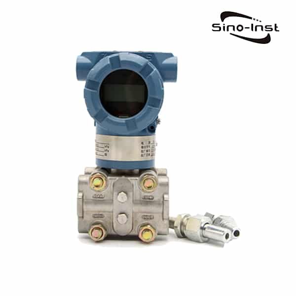
A differential pressure transmitter (DPT) measures the pressure drop across two points — across an orifice for flow, across a liquid column for level, or between two process taps for filter monitoring. Installation decides whether the published 0.075% accuracy survives in the field or drifts within a week. This guide gives the service-specific hook-up rule, concrete impulse-line slope and length numbers, manifold selection, and the post-mount zero/range procedure used by Sino-Inst commissioning engineers.

Contents

Pre-Install Checklist for DP Transmitters

Before the transmitter leaves the panel shop, three numbers should be locked down: the calibrated range (e.g. 0–250 inH₂O), the static line pressure rating, and the output type (4–20 mA HART, FF, Profibus PA). Range turndown beyond 10:1 erodes accuracy on most silicon DPTs; pick a sensor module sized closer to the working span, not the worst case. Confirm whether the service needs a wet leg or a dry leg — this drives whether you order remote-seal diaphragms or a standard process flange.

Field accessories that ship with a clean DPT installation: a process manifold (almost always required), a 2-inch pipe stand or wall bracket for direct mount, signal cable rated for the area classification, weather-tight conduit fittings, and seal/blow-down valves on each impulse leg. Pulling cable through a damp tray six weeks after pressure-testing is the most common avoidable callback. See our pressure transmitter installation guide for shared electrical practices that apply here too.

Hook-Up by Service: Gas, Liquid, Steam, Level

The single rule that decides DPT mounting position is: keep the impulse fluid in a known, stable phase. That single principle drives four very different installations. After installation, perform the 5-point calibration check before commissioning the loop.

ServiceMount the transmitterTap location on the lineWhy
Gas (flow / DP)Above the process tapTop of the pipeAny condensate drains back to the line; the impulse legs stay full of gas at the same density
Clean liquidBelow the process tapSide of the pipe (3 o’clock or 9 o’clock)Trapped gas migrates up into the line, not into the legs; legs stay full of liquid
SteamBelow the tap, with condensate pots at the tapsSide of the pipe at each tap, with sealing pots installed at the same elevationThe pots fill with condensate and protect the transmitter diaphragm from live steam
Liquid level (open / closed tank)At or below the lower tap (HP side)HP on lower tank nozzle; LP on upper nozzle or vented to atmosphereHydrostatic head is measured directly; closed tanks need a wet or dry leg compensation

For orifice plate flow, also enforce the upstream/downstream straight run before measurement. A DPT installed too close to an elbow reads correctly but the orifice no longer does. Our reference on flow meter straight pipe requirements lists the 10D upstream / 5D downstream rule and the exceptions by meter type. For broader sizing math, see our note on flow rate and pressure.

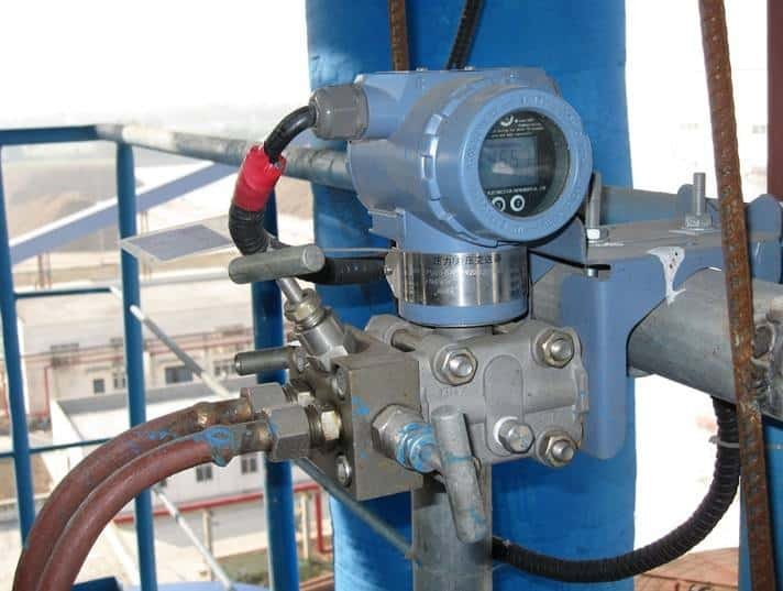
Differential pressure level transmitter installed on a tank with HP and LP impulse lines

Impulse Line Routing Rules

Concrete numbers, not “slope properly”:

  • Slope: 1:12 minimum (about 1 inch per foot, or 8 cm per meter) continuously toward either the transmitter (liquid service) or the process (gas service). No flat runs, no inverted U-bends.
  • Maximum length: 50 ft (15 m). Longer runs drag dynamic response above 1 second and amplify temperature error on the legs.
  • Both legs equal: within ±10% in length. Unequal legs introduce a temperature-driven zero shift you will chase forever.
  • Inside diameter: 1/2 in (12 mm) for most services. Step up to 3/4 in for viscous liquids or long runs.
  • Heat tracing & insulation: required when freezing, condensation, or viscosity change is possible. Trace both legs identically.
  • Drain / vent valves: one drain at the low point of liquid legs, one vent at the high point of gas legs. Use these during commissioning, not just for maintenance.

If the line includes a known restriction or filter, the pressure drop in the pipe needs to be in the same range as the transmitter’s calibrated span; otherwise the signal saturates or under-resolves.

Manifold Selection: 3-Valve vs 5-Valve

The manifold is the single accessory that decides whether the field tech can safely zero a transmitter under process pressure. Three configurations are common:

  • 3-valve manifold: two block valves (HP, LP) plus one equalize. Sufficient for non-hazardous, low-pressure services up to about ANSI 600. Equalize-isolate sequence: close HP block → open equalize → close LP block → vent → zero.
  • 5-valve manifold: adds two vent/test ports. Required for high-static or hazardous service, and for any line where the transmitter will be re-zeroed live without draining. The extra ports let the tech bleed isolated air and verify the equalize seal before applying full DP.
  • Remote diaphragm seals: not a manifold but worth flagging here. On corrosive, hot, or viscous services, capillary-coupled seals replace impulse lines entirely. Order with matched capillary length and fill fluid suited to ambient swings.

Zero & Range After Mounting

Five steps, in this order, every time:

  1. Close both block valves. Open the equalize valve. The DPT now sees zero differential pressure regardless of static line pressure.
  2. Vent each side individually if the manifold has vent ports. Confirm legs are full of process fluid (liquid service) or process gas (gas service).
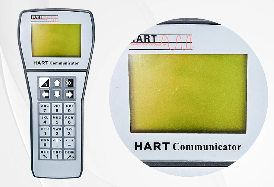
  3. Apply the zero command — locally via the push-button, or remotely via HART, FF, or Profibus.
  4. Close the equalize valve. Open the LP block, then the HP block. The transmitter is now live.
  5. Verify the 4–20 mA span with a pressure calibrator across at least three points (0%, 50%, 100% of range). Trim the output if needed via the digital communicator.

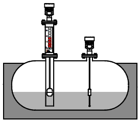
For closed-tank level service, apply the wet-leg correction at this stage. The LP leg holds a column of seal fluid (often glycol or silicone). The correction is ρ·g·h where ρ is the seal fluid density, g is 9.81 m/s², and h is the vertical distance between the LP tap and the transmitter. The HART or BRAIN command for “lower-range value” lets you bake the correction into the calibration without changing wiring. If you need a refresher on the wiring, the 4–20 mA loop conversion guide covers the receiving side.

Common Installation Mistakes

  • Mixing HP and LP labels. Reverse polarity reads as a negative span. Verify with a manual squeeze test on each leg before energizing.
  • Trapped air in liquid legs. Manifests as drift on every static line pressure change. Bleed thoroughly during commissioning; vent again after the first week.
  • Condensate in gas legs. Common on saturated process gas. Slope toward the line, not the transmitter, and add a knock-out pot if the gas trips dew point seasonally.
  • Capillaries exposed to direct sun. Temperature gradient across the two capillaries introduces a zero shift that tracks daylight. Sun-shield both capillaries identically.
  • Mounting on a vibrating pipe. Bracket-mount to a structural support, not the pipe itself. Vibration above ~1 g RMS damages the silicon diaphragm bond over months. Our note on pressure transmitter vs gauge selection covers durability trade-offs.
  • Ignoring static line pressure spec. A DPT calibrated for 250 inH₂O on a 1000 psi static line needs the static rating. Exceeding the static spec damages the sensor module silently. The static vs dynamic vs total pressure explainer shows where each value comes from.

Featured DP Transmitters from Sino-Inst

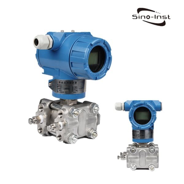
SMT3151DP Smart DP Transmitter

0.075% accuracy | 4–20 mA HART | up to 32 MPa static — single-crystal silicon sensor for flow, level, and filter DP service.

Flange-Mounted DP Transmitter

Direct flange mount with remote diaphragm seal option — eliminates impulse lines on hot, viscous, or corrosive process services.

SMT3151LT DP Level Transmitter

Hydrostatic level for open and closed tanks — built-in wet/dry-leg compensation, IP67 housing, ATEX/IECEx options.

FAQ

How do you install a differential pressure transmitter?

Mount the transmitter relative to the process per service (gas above, liquid below, steam below with condensate pots, level at or below the lower tap). Route both impulse legs at a minimum 1:12 slope toward the correct direction, install a 3- or 5-valve manifold, and finish with the equalize-zero-span sequence using a HART or 4–20 mA calibrator.

What is the difference between DPS and DPT?

A differential pressure switch (DPS) trips a discrete contact when DP crosses a set threshold. A differential pressure transmitter (DPT) outputs an analog or digital signal proportional to DP across the full range, so it feeds control loops and trending systems rather than only alarms.

Why install a DP transmitter above the tap point for gas?

On gas service, any condensate that forms in the impulse legs must drain back to the process line, not into the transmitter. Mounting above the taps, with the legs sloped downward toward the line, lets gravity remove condensate continuously and keeps both legs filled with gas at the same density.

What straight pipe is needed upstream and downstream of an orifice?

ISO 5167-2 lists upstream straight runs from roughly 5D to 44D depending on β ratio and the upstream fitting (single elbow, two elbows in different planes, reducer, valve). Downstream is generally 4D to 8D. A safe baseline on most plant configurations is 10D upstream and 5D downstream, with longer upstream runs after two elbows in different planes. See our straight pipe requirements table for the exceptions.

Need help sizing a DPT, picking between a 3-valve and 5-valve manifold, or specifying remote seals for a hot process line? Send your service conditions to our engineering team and we will quote a complete installed scope.

Request a Quote

Please enable JavaScript in your browser to submit the form

Flow Rate and Pressure: Formula, Worked Example & Conversion Table

Flow rate and pressure are linked by Bernoulli’s equation, by friction losses, and by the geometry of whatever the fluid passes through. A pump that delivers 200 kPa across a 50 mm pipe will not push the same volume per minute as one delivering 200 kPa across a 25 mm pipe. Pressure alone is not flow — and flow alone is not pressure. The rest of this page walks through the formulas you actually use in the field, two worked examples, and the corrections every engineer needs to apply when reading a flow meter spec from a vendor.

Contents

How Flow Rate and Pressure Relate

Pressure is the energy per unit volume that drives a fluid; flow rate is how much volume crosses a section in a given time. They are tied by three physical realities:

  • Energy conservation. Bernoulli’s equation says total head — pressure + velocity + elevation — is conserved along a streamline (ideal case). Drop the pressure across an orifice and the velocity (hence flow) rises.
  • Friction loss. Real pipes consume pressure to push the fluid against wall shear. Doubling the flow roughly quadruples the friction loss in turbulent flow.
  • Geometry. Pipe diameter, roughness, fittings, and the restriction itself (orifice, valve, nozzle) determine how much flow a given pressure differential produces.

The Five Core Formulas

Keep these five formulas on a card next to your desk. They cover 90% of plant calculations.

Use caseFormulaNote
Bernoulli (ideal)P + ½ρv² + ρgh = constantConservation along a streamline, no friction
Orifice / Venturi (incompressible)Q = Cd · A · √(2ΔP / ρ)The workhorse for DP-based flow measurement
Darcy-Weisbach (pipe friction)ΔP = f · (L/D) · (ρv²/2)Friction factor f from Moody chart
Hagen-Poiseuille (laminar flow)Q = (Π · ΔP · D⁴) / (128 · μ · L)Valid for Re < 2300; very small pipes/oils
Valve / restriction (Cv coefficient)Q = Cv · √(ΔP / SG)Flow in GPM, ΔP in psi, SG specific gravity

Two practical notes. The orifice formula uses ΔP (pressure differential), not absolute line pressure — a transmitter reporting 5 bar of line pressure tells you nothing about flow unless you also know the upstream-to-downstream drop. And the Cv formula is unit-bound: psi and GPM are required as input, not bar and m³/h. Convert before using or read our differential-pressure flow calculator walkthrough for a SI-unit version.

Worked Example — Calculating Flow from Pressure

An orifice plate sits in a 100 mm horizontal water line. Bore diameter is 60 mm. The DP transmitter reads 25 kPa. Find the flow rate.

If your pump curve is in LPM but the procurement spec is in US gallons per minute, run a sanity check on the conversion before sizing — our LPM to GPM conversion guide covers the US/UK gallon gap and the spec-sheet decoder.

  1. Beta ratio β = d/D = 60/100 = 0.6.
  2. For β = 0.6 in turbulent water flow, discharge coefficient Cd ≈ 0.62 (ISO 5167 table).
  3. Orifice area A = π · (0.06/2)² = 2.827 × 10⁻³ m².
  4. Water density ρ = 1000 kg/m³. ΔP = 25,000 Pa.
  5. Q = 0.62 · 2.827e-3 · √(2 · 25000 / 1000) = 0.62 · 2.827e-3 · 7.07 = 0.01239 m³/s.
  6. Convert to working units: 0.01239 m³/s × 3600 = 44.6 m³/h, or about 196 GPM.

The same 25 kPa drop across a different bore would give a different flow. That dependence on geometry is why DP flow meters need a calibration certificate that matches the installed bore and pipe, not just the spec sheet’s claimed accuracy. See straight-run pipe requirements for the installation rules that keep the calibration valid.

Pressure Drop in Real Piping

The total pressure loss in a real pipe run is the sum of friction in straight pipe plus losses at every fitting. A simplified working form:

  • Straight pipe loss: Darcy-Weisbach (above). Friction factor f rises with roughness and falls with Reynolds number.
  • Fitting losses: ΔPfitting = K · (ρv²/2). K values from tables — 90° elbow K ≈ 0.75, gate valve fully open K ≈ 0.15, sudden contraction K ≈ 0.5.
  • Elevation: ρgh — 1 m of water adds 9.81 kPa to the static head requirement.

The friction line on a pump curve is the sum of these terms. When the pump’s pressure output equals the system’s friction demand at a given flow, the system stabilises at that operating point. Most underperforming pump installations trace back to a friction estimate that ignored elbows, valves, or the eventual fouling-up of strainers and heat exchangers.

Why the Pressure-Flow Curve Matters for Pump Selection

A centrifugal pump produces more flow at lower pressure and less flow at higher pressure. Plot the pump’s pressure-vs-flow curve on the same axes as the system’s friction curve. The intersection is the operating point.

  • If the system curve drifts left of the pump’s best efficiency point (BEP), you waste energy and risk recirculation damage.
  • If the system curve sits right of BEP, the motor may overload during low-resistance conditions (filter clean, valve open).
  • Aim to size pumps so the design point sits within ±10% of BEP, then verify with a flow meter K-factor calibration after commissioning.

Quick Reference Table — Pressure to Flow

Approximate flow through a 1″ (25 mm) clean steel pipe, water at 20 °C, no fittings, fully developed turbulent flow. Use as a sanity check, not a design value.

Line pressure (psi)Approx. flow (GPM)Approx. flow (m³/h)
10143.2
20204.5
40286.4
60347.7
80409.1
1004410.0

Note the non-linearity. Doubling pressure does not double flow because friction losses scale with v² — about 40% more pressure is needed to move twice the volume. Engineers used to volumetric scaling are often surprised by how badly bigger pumps underperform expectations.

Common Mistakes Calculating Flow from Pressure

  • Confusing absolute pressure with differential pressure. Line pressure tells you nothing on its own — flow follows the DP across a known restriction.
  • Ignoring fluid properties. Hot water has a different viscosity and density from cold water. A static vs dynamic pressure check matters before reaching for Bernoulli.
  • Assuming the orifice Cd is 1.0. Real coefficients run 0.6 to 0.8 depending on beta ratio and Reynolds number. ISO 5167 lists actual values.
  • Mixing units. The Cv formula needs psi and GPM. The orifice formula needs SI units. Convert before substituting.
  • Forgetting upstream straight-run. An orifice that meets ISO 5167 in the lab but sits 1 D downstream of a 90° elbow on site will read 5-10% off true flow. Read the magnetic flow meter installation guide for similar straight-pipe rules across meter families.

Featured DP Flow Meters and Pressure Transmitters from Sino-Inst

Industrial Magmeter Flow Meters

DN6-DN3000 | 4-20 mA, pulse, Modbus | conductive liquids — measures flow directly, no DP calculation needed.

SMT3151DP Differential Pressure Transmitter

100:1 turndown | 0.075% accuracy | HART + 4-20 mA — pair with an orifice plate to compute Q from ΔP.

Verabar Averaging Pitot Tube

Insertion design | low permanent pressure loss | DP output for air, gas, steam, water — minimal installation cost.

Frequently Asked Questions

What is the formula for flow rate from pressure?

For a fluid passing through a restriction: Q = Cd · A · √(2ΔP / ρ). ΔP is the pressure drop across the restriction, A is the restriction area, ρ is the fluid density, and Cd is the discharge coefficient (typically 0.6 to 0.8 for orifices).

Does higher pressure always mean higher flow?

No. Higher line pressure does not by itself produce more flow. Flow rises when the pressure differential across the system increases, while the system geometry stays constant. A sealed pipe at 10 bar has zero flow despite high pressure.

How do I convert pressure to flow rate in GPM?

The simplest practical conversion uses the valve coefficient: Q (GPM) = Cv · √(ΔP / SG), where ΔP is in psi and SG is specific gravity. For pipes without a defined restriction, you need pipe length, diameter, roughness, and fluid properties — there is no single-number conversion.

What is Bernoulli’s equation used for?

Bernoulli’s equation conserves total energy (pressure + kinetic + potential) along a streamline for an ideal fluid. In instrumentation, it underpins the orifice, venturi, and pitot-tube flow-measurement formulas. Real-world calculations correct Bernoulli with a discharge coefficient or friction term.

Why does my flow meter read low at high pressure?

Several causes. A DP meter on an orifice reads correctly only within its calibrated turndown — extreme pressure drops outside that range introduce nonlinearity. Or the pressure is compressing a gas, so volumetric flow shrinks even though mass flow is steady. Check the meter’s calibration certificate and whether the reading is volumetric or mass-based.

Sino-Inst engineers have specified flow elements, DP transmitters, and magnetic and ultrasonic flow meters for refineries, water utilities, and chemical sites across more than 50 countries. Send the line size, fluid properties, and the pressure range — the team will return a sized configuration. Learn more about the Sino-Inst engineering team and request a quote below.

Request a Quote

Please enable JavaScript in your browser to submit the form

What Does SCADA Stand For? Supervisory Control And Data Acquisition Explained

SCADA stands for Supervisory Control And Data Acquisition. It is the software-and-hardware stack that lets one operator watch — and steer — dozens or hundreds of field instruments from a single screen. SCADA does not run the loop itself; PLCs and RTUs do. SCADA sits on top, pulling tags, drawing trends, raising alarms, and writing back setpoints. The five letters describe what the system is for, in that order: Supervisory first, Acquisition last. The rest of this page explains each part, where SCADA earns its keep, and where another tool would fit better.

Contents

SCADA Spelled Out — Supervisory Control And Data Acquisition

The acronym dates to the 1960s utility industry, when a single dispatcher first needed a screen view of dozens of remote pumping stations. Every letter still earns its place on a modern P&ID.

LetterWordWhat it means on the floor
SSupervisoryOne operator oversees many controllers; SCADA does not replace local logic.
CControlOperator can write setpoints, open/close valves, start/stop pumps from the HMI.
AAndConjunction — included so the acronym reads as English.
DDataTag values (temperature, flow, level, status bits) polled or streamed from the field.
AAcquisitionThe act of pulling those tags into a historian for trending, reporting, alarms.

Two utilities deserve emphasis. Supervisory means SCADA is a layer above the controllers — strip the SCADA away and the plant still runs on the PLC’s ladder logic. Acquisition means the system is, at its core, a data-pulling engine; visualization and alarms are downstream of that pull.

The Five Building Blocks of a SCADA System

Every SCADA installation, from a two-pump booster station to a national gas pipeline, breaks down into the same five layers.

  1. Field instruments. Sensors and transmitters that convert physical state to a 4-20 mA, HART, or digital signal. A typical plant has hundreds — flow meters, pressure sensors, level probes, thermocouples, gas detectors.
  2. RTUs and PLCs. Microprocessor controllers that read the field signals, run local logic (interlocks, simple PID), and forward tag values upstream. RTUs are typically remote and ruggedized; PLCs are typically inside the plant cabinet.
  3. Communication network. The transport layer — Modbus RTU/TCP, OPC UA, DNP3, Ethernet/IP, cellular, or radio. The choice depends on distance, determinism, and security posture.
  4. Master Terminal Unit (MTU). The supervisory server. It maintains the tag database, runs the historian, evaluates alarms, and pushes setpoints back to the RTUs.
  5. Human-Machine Interface (HMI). The operator screens. Mimic diagrams, trends, alarm banners, login profiles. The HMI is the face of SCADA; the MTU is the brain.

How SCADA Works in a Real Plant

The signal flow is bidirectional but asymmetric. Data goes up almost continuously; commands come down only when an operator (or a script) asks. A typical polling cycle looks like this:

  • Every 1-5 seconds, the MTU sends a Modbus or DNP3 read to each RTU.
  • The RTU returns the current tag values — flow in m³/h, pressure in bar, valve position, motor status.
  • The MTU stamps the values, archives them in the historian, evaluates each against the alarm limits, and updates the HMI screens.
  • If an operator writes a new setpoint or clicks a “Start Pump” button, the MTU pushes a Modbus write to the RTU. The RTU passes the command to the PLC, which executes the change in the next scan.

A common field surprise: SCADA does not close fast loops. Anything tighter than ~100 ms — pressure relief, motor protection, surge control — has to live in the PLC. The SCADA layer is for shift-scale supervision, not millisecond control. Pair SCADA with a tuned PID controller in the PLC, not the other way around.

SCADA vs PLC vs DCS — Decision Matrix

The three terms are not interchangeable, though every vendor’s marketing tries to blur them. Use this matrix when choosing:

AttributePLCSCADADCS
Primary purposeLocal logic executionSupervisory visualization & dataPlant-wide integrated control
Loop speed1-50 ms scan1-5 s polling50-500 ms
OrientationDiscrete, machine-levelData-centricContinuous, process-centric
ScopeOne machine / cellSite to enterpriseOne plant, deeply integrated
Typical fitConveyor, batch skidWater utility, pipeline, multi-siteRefinery, chemical plant
Capex / loopLowLow to mediumHigh

The most common production architecture is PLC + SCADA. PLCs handle the millisecond control; SCADA sits on top to show, log, and supervise. A DCS replaces both layers with one integrated stack — that integration costs more and only pays back in tightly coupled continuous processes.

Where SCADA Earns Its Keep — Cross-Industry Snapshot

SCADA shows up wherever assets are dispersed and a small team needs visibility across all of them.

  • Water and wastewater. Lift stations, treatment plants, reservoirs. Tags from magnetic flow meters and submersible level probes converge to one control room.
  • Oil and gas. Pipeline pressure, custody-transfer flow, tank pressure measurement, RTU-equipped wellheads. SCADA over satellite or cellular keeps thousands of kilometers under one screen.
  • Power transmission. Substation breaker status, transformer temperatures, line currents. SCADA in this domain is sometimes called EMS (Energy Management System) but the SCADA layer underneath is the same.
  • Food and beverage. Clean-in-place (CIP) cycles, fermenter temperatures, batch tracking and differential-pressure flow totalization. SCADA enforces recipe steps and writes batch records for audit.

A unifying pattern: SCADA pays back fastest when the cost of one operator walking the site exceeds the cost of one Modbus radio. That ratio is why utilities adopted SCADA decades before light manufacturing did.

Common Misreadings of “SCADA”

Two misreadings show up regularly in spec documents and interview questions.

  • NOT “Sequential Control And Data Acquisition”. Sequential control belongs to a PLC running batch logic. SCADA is supervisory — above the sequence, not inside it.
  • NOT “System Control And Data Acquisition”. “System” is generic and obscures the hierarchical meaning. The word is “Supervisory” deliberately, signaling that SCADA observes and overrides without owning the local loop.

The distinction is not pedantic. Auditors, NIST cybersecurity guidance, and ISA-95 all use “Supervisory” — getting the word wrong on a tender response signals limited familiarity with the architecture.

When SCADA Is the Wrong Tool

SCADA is not always the answer. Three situations where a different layer fits better:

  • Single-machine logic. A standalone packaging machine with a local HMI does not need a supervisory layer. A PLC plus a panel-mount HMI is cheaper and more reliable.
  • High-integration continuous processes. A modern olefins plant or large refinery wants a DCS, where control and supervision share the same engineering database. Bolting SCADA onto bare PLCs in that setting creates integration debt.
  • Lightweight IIoT pilots. If the goal is to push a dozen sensors to a cloud dashboard for energy benchmarking, a modern edge gateway plus a cloud time-series database is faster to stand up than a SCADA install. SCADA returns to the picture once control writes are required.

Spec-Sheet Decoder — Acronyms You’ll See Around SCADA

AcronymStands forWhere you meet it
RTURemote Terminal UnitRuggedized field controller, often at the well or lift station
PLCProgrammable Logic ControllerIn-plant logic execution, fast scan
HMIHuman-Machine InterfaceOperator screen — panel-mount or PC-based
MTUMaster Terminal UnitThe supervisory server in the SCADA stack
IEDIntelligent Electronic DeviceSubstation protective relay with embedded logic
ICSIndustrial Control SystemUmbrella term covering SCADA + DCS + PLC
OPC UAOpen Platform Communications Unified ArchitectureModern interoperability protocol

Most of these terms appear together in vendor datasheets and standards documents. ISA-99 and IEC 62443 treat them all under “industrial control systems” for cybersecurity purposes.

Sensors and Transmitters That Feed SCADA

Every SCADA tag traces back to a physical instrument. The three product families below are typical inputs to a SCADA layer at a water, oil & gas, or chemical site.

SMT3151 Gauge Pressure Transmitter

4-20 mA + HART | 0.075% accuracy | -40 to 85 °C — direct loop into SCADA RTU or PLC analog input card.

Industrial Magmeter Flow Meters

DN6-DN3000 | 4-20 mA, pulse, Modbus | conductive liquids — workhorse flow tag for water and wastewater SCADA.

Radar Water Level Sensor

0.05 m to 120 m range | non-contact 80 GHz FMCW | 4-20 mA + HART — reliable tank, river and reservoir level for remote SCADA stations.

Frequently Asked Questions

What does SCADA stand for in PLC discussions?

The acronym is the same — Supervisory Control And Data Acquisition. In a PLC-centric conversation, “SCADA” refers specifically to the software layer above the PLC that visualizes tags and logs data. The PLC runs the loop; SCADA watches it.

Is SCADA the same as HMI?

No. The HMI is one component of a SCADA system — the operator-facing screen. SCADA also includes the historian, alarm engine, tag database, and communication drivers to the RTUs. A panel-mount HMI on a single machine is not SCADA.

Is SCADA part of IIoT?

SCADA predates IIoT by decades, but the two overlap. Modern SCADA platforms expose tags via OPC UA or MQTT and feed cloud dashboards, which is functionally IIoT. The difference is intent: SCADA owns the control authority; IIoT platforms typically do not write back to the field.

Who invented SCADA?

No single inventor — the concept evolved through the 1960s and 1970s among electric utilities and oil pipeline operators who needed centralized telemetry. Early systems used dedicated minicomputers and proprietary telemetry; the term “SCADA” itself was in common use by the mid-1970s.

What language do SCADA systems use?

Two layers, two languages. The PLCs underneath use IEC 61131-3 languages — ladder logic, structured text, function block. The SCADA software itself is typically configured graphically; scripting, when needed, is in VBScript, Python, or vendor-specific languages.

Sino-Inst engineers have specified SCADA-ready instrumentation for water utilities, oil & gas terminals and chemical sites across more than 50 countries. If you are scoping a new SCADA tag list — or replacing legacy field instruments that no longer match modern protocols — contact our team for a sized quote and protocol checklist. Learn more about the Sino-Inst engineering team and request a tailored configuration below.

Request a Quote

Please enable JavaScript in your browser to submit the form

Pressure Transmitter Working Principle: 6 Sensing Technologies & 5 Types

A pressure transmitter converts process pressure into a 4-20 mA, HART, or digital signal that a control system can read. Inside the housing, a sensing element deflects under pressure; the deflection is measured as a change in resistance, capacitance, or frequency; analog circuitry conditions and scales the signal; and an output stage drives the loop. The rest of this guide walks through the six sensing technologies in use today, the five common transmitter types you will see on a P&ID, how to read the accuracy line on a spec sheet, and the field installation mistakes that quietly cost accuracy. When the receiving PLC expects a voltage instead of a current loop, you can convert the 4-20 mA signal to 0-10 V using a precision resistor.

Process transmitters measure static pressure at the diaphragm — for the difference between static, dynamic, and total pressure, and how Pitot probes read each, see our static vs dynamic vs total pressure guide.

Contents

Working Principle in 60 Seconds

Process pressure pushes on a diaphragm. The diaphragm deflects — typically by micrometres. A sensing element behind the diaphragm reports that deflection as a change in electrical property: resistance for piezoresistive bridges, capacitance for capacitive cells, frequency for resonant sensors. An ASIC linearises and temperature-compensates the reading, then drives a current loop output proportional to applied pressure.

The classic span is 4 mA at 0% of range, 20 mA at 100%. The live-zero (4 mA, not 0 mA) is deliberate: it lets the receiver distinguish a true zero-pressure reading from a broken loop wire. Engineers have leaned on that convention since the 1950s.

Six Pressure Sensing Technologies

Different sensing elements suit different working ranges, fluids, and accuracy targets. Engineers can also reference the full list of common pressure units when setting transmitter ranges.

TechnologyHow it worksTypical accuracySweet spot
Piezoresistive (strain gauge)Diffused silicon resistors form a Wheatstone bridge on the diaphragm; pressure changes resistance±0.075% to ±0.25%General industrial, oil & gas, HVAC
CapacitiveDiaphragm forms one plate of a capacitor; deflection changes capacitance±0.025% to ±0.075%Custody transfer, low-DP measurement
Resonant (silicon)Pressure changes the natural frequency of a vibrating silicon beam±0.04% to ±0.1%High-stability subsea and fiscal metering
PiezoelectricQuartz or PZT crystal generates charge under stress±0.1% to ±0.5%, dynamic onlyEngine combustion, ballistic, impact
Optical (fibre)Pressure changes the wavelength reflected from a Bragg grating±0.05% to ±0.2%EMI-noisy substations, downhole
Inductive / LVDTDiaphragm moves a magnetic core inside a coil±0.25% to ±0.5%Rugged hydraulic and pneumatic service

Piezoresistive sensors win most general-purpose specifications on price, while capacitive sensors take over when accuracy specs go below ±0.05%. Optical fibre transmitters are a recent entrant into hazardous-area and downhole oil & gas use, where electromagnetic isolation justifies the cost. For the field installation procedure with hook-up by service, manifold selection, and zero/range steps, see our DP transmitter installation.

Five Pressure Transmitter Types on a P&ID

  1. Gauge Pressure (PG, PT). Reference to atmospheric. Most common type for tank levels, pump discharge, hydraulic systems. Range 0-1 bar through 0-700 bar.
  2. Absolute Pressure (PA). Reference to vacuum. Used in vacuum process, vapour pressure, altitude, and barometric correction. Range 0-1.6 bar abs to higher.
  3. Differential Pressure (DP). Two process ports; transmitter reports the difference. Flow elements (orifice, venturi), filter monitoring, and DP-level transmitters all use this class.
  4. Multivariable. One transmitter outputs flow, DP, static pressure, and temperature simultaneously. Used in fiscal metering and natural-gas custody transfer.
  5. Remote Seal / Diaphragm Seal. Capillary-coupled fill fluid isolates the sensor from corrosive, hot, or viscous media. Found on glycol service, polymer reactors, food & pharma.

Signal Outputs Decoded

The transmitter is only as useful as the receiver it talks to. Match the output protocol to the control hierarchy. For step-by-step bench calibration including HART sensor and D/A trim, see our pressure transmitter calibration procedure.

  • 4-20 mA analog. The lingua franca. Two-wire, loop-powered, immune to voltage drop. Pairs with any PLC analog input card.
  • 4-20 mA + HART. A digital sideband on the same two wires. Lets a HART handheld read diagnostics, ranges, and tags without breaking the loop.
  • Modbus RTU / RS-485. Multi-drop digital. Best for retrofits and substation/water-utility installations where a SCADA historian reads dozens of tags from one cable.
  • FOUNDATION Fieldbus / PROFIBUS PA. Native-fieldbus protocols. Lower wiring counts but require trained engineering and a fieldbus power supply.
  • Wireless HART, ISA100. For remote tanks, rotating equipment, and brownfield additions where pulling cable is uneconomic.

Most greenfield projects still default to 4-20 mA with HART superimposed. The combination keeps the analog signal robust for safety loops while exposing diagnostics on demand. Read more on how signal-output choices affect transmitter selection.

Engineering Selection Checklist

Walk a specification request from process data sheet to purchase order using these eight checks:

  1. Measured variable. Gauge, absolute, differential, or compound? Pick before anything else.
  2. Operating range. Place normal operating pressure between 25% and 75% of full scale. Overranging the top end shortens diaphragm life; undersizing kills accuracy.
  3. Required accuracy. Match to the loop need: ±0.5% for general utility, ±0.1% for safety loops, ±0.025% for custody transfer.
  4. Wetted materials. 316L for clean water and air; Hastelloy C, Monel, or tantalum for chlorides, sulphuric, and fluorinated streams.
  5. Process connection. 1/2″ NPT, G1/2″, or DIN flange — confirm against the existing tap.
  6. Output protocol. Decide before specifying — see the section above.
  7. Hazardous-area certificates. ATEX, IECEx, CSA, FM. Get the Ex-d or intrinsically safe variant if the area zone requires it.
  8. Ambient + process temperature. Plain transmitters run -40 to 85 °C ambient; remote seal extends process side to 400 °C with the right fill fluid.

For a deeper look at how transmitters differ from mechanical gauges, see pressure transmitter vs pressure gauge — different categories of instrument that look similar from outside but behave very differently in service.

Common Installation Mistakes

  • Impulse line freezing. Outdoor lines on winter service need heat-tracing or a diaphragm seal. A frozen line reads constant or wildly noisy.
  • Pulsation on positive-displacement pumps. Install a needle-valve snubber or pulsation dampener. Without one, the sensor sees 10× the true mean and ages prematurely.
  • Mounting orientation on remote seals. Capillaries fight gravity; mounting the seal above the transmitter on a long capillary introduces a head-pressure offset that drifts with ambient temperature.
  • Single-isolation valve on safety service. Three-valve manifolds for DP, five-valve for SIL-rated service. Single-valve installs cannot be safely zeroed in-line.
  • Vent / drain neglect. Liquid lines on gas service need a high vent; gas lines on liquid service need a low drain. Trapped air or condensate gives a +/- offset that operators chase for shifts.

Spec-Sheet Decoder

Spec lineWhat it really means
±0.075% of spanBest-fit straight-line accuracy across full calibrated span. Worst case at endpoints.
±0.04% URLRefers to the Upper Range Limit (URL), not the calibrated span. Often better than “of span” at low ranges.
BFSLBest Fit Straight Line — the linearity method behind “%” accuracy. Tighter than terminal-based.
Turndown 100:1You can calibrate the transmitter at 1% of URL and still keep stated accuracy. Useful for stocking spares.
Long-term stability ±0.1%/5 yrDrift you should expect between calibration cycles.
EMC IEC 61326The transmitter passes industrial EMC immunity — important on VFD-rich plants.

Featured Pressure Transmitters from Sino-Inst

SMT3151 TGP Gauge Pressure Transmitter

4-20 mA + HART | 0.075% accuracy | -40 to 85 °C — the workhorse Sino-Inst gauge transmitter for general process service.

Diaphragm Seal Pressure Transmitters

Capillary-coupled seal | flush, extended, or remote diaphragm | corrosion and high-temperature service to 400 °C.

SMT3151DP Smart Differential Pressure Transmitter

100:1 turndown | 0.075% accuracy | HART + 4-20 mA — DP across orifice, filter, or for tank-level applications.

Frequently Asked Questions

How does a pressure transmitter work in simple terms?

Process pressure flexes a thin metal diaphragm by a few micrometres. A sensing element behind the diaphragm — typically a piezoresistive bridge or a capacitive cell — converts that flex into an electrical signal. Onboard electronics linearise, temperature-compensate, and scale the signal to a 4-20 mA loop output that any control system can read. For background on the wetted parts list, see our materials guide.

What is the difference between a pressure transmitter and a pressure sensor?

The sensor is the raw element — the silicon strain bridge or ceramic capacitive cell. The transmitter is the sensor plus signal conditioning, temperature compensation, EMC filtering, and a standard process output. Sensors live inside transmitters; you wire transmitters into plant control.

What does “smart” pressure transmitter mean?

A smart transmitter has a microprocessor on board. It supports HART digital communication for ranging and diagnostics, applies multi-point temperature and linearity correction internally, and stores its own tag and calibration record. Non-smart (analog) transmitters trim by potentiometer and have no digital sideband.

How accurate is a typical industrial pressure transmitter?

General-purpose units sit at ±0.075% to ±0.25% of calibrated span. Custody-transfer transmitters reach ±0.025%. Below that you are buying a metrology-grade instrument, not a process transmitter.

Can I use one pressure transmitter for level measurement?

Yes. Static head in a vented tank is directly proportional to liquid level when density is known; a gauge transmitter mounted at the bottom of the tank reads level via P = ρgh. Pressurised tanks need a differential pressure transmitter to subtract head-space pressure. See the SMT3151LT DP level transmitter for that application.

Sino-Inst engineers have specified pressure transmitters for refineries, water utilities, chemical plants, and pharmaceutical sites across more than 50 countries. Send your process data sheet — span, accuracy, wetted material, process connection — and the team will return a sized configuration with delivery and certificate package. Read more about the Sino-Inst engineering team and request a quote below.

Request a Quote

Please enable JavaScript in your browser to submit the form

BTU Meter for Chilled Water: Ultrasonic vs Magnetic + Worked Calculation

Updated Apr 25, 2026 — Reviewed by Sino-Inst Engineering Team

A BTU meter for chilled water quantifies cooling energy by combining a flow meter with a matched pair of RTDs on the supply and return. On a typical HVAC loop at 44°F supply / 54°F return (10°F ΔT), the temperature signal — not the flow signal — drives almost all of the billing-grade uncertainty. This guide covers ultrasonic vs electromagnetic selection, why ±0.1°F matched PT1000 pairs are non-negotiable, straight-pipe rules, and BACnet / Modbus integration. For the primer, see What Is a BTU Meter.

Contents

How a BTU Meter Works for Chilled Water

A BTU meter integrates three signals into one energy totalizer: volumetric flow (ṃ), fluid specific heat (cp), and the return-minus-supply temperature difference (ΔT). The governing equation is:

The flow input is volumetric — converted from LPM, m³/h, or GPM into the totalizer’s internal unit. If a spec is in litres per minute but the BMS expects gallons per minute, our LPM to GPM conversion reference gives the exact factor and the US/UK gallon caveats.

Qenergy = ṃ × cp × ΔT

For a chiller plant delivering 500 GPM at 10°F ΔT, that is roughly 2.5 million BTU/hr (about 208 tons). For pulse-output flow meters, the integrator also stores the K-factor (see our flow meter K-factor chart for typical values). The integrator samples flow and both RTDs once per second and totalizes energy in BTU, kWh, MJ, or ton-hours.

The error budget is dominated by ΔT, not flow. At a 10°F design ΔT, a 0.2°F combined RTD error is a 2% energy error. At part-load — where chilled-water plants spend most run hours — ΔT collapses to 5–6°F and the same RTD error costs 3–4%. A ±0.5% flow meter cannot rescue a sloppy RTD pair, regardless of the underlying flow-rate vs pressure relationship in the loop.

Ultrasonic vs Electromagnetic BTU Meters for Chilled Water

Two technologies dominate chilled-water BTU metering. Transit-time Ultrasonic Water Flow Meters measure the time difference of acoustic pulses travelling with and against flow — no wetted parts, no pressure drop, clamp-on variants install without shutdown. Electromagnetic meters apply Faraday’s law and need fluid conductivity above 5 µS/cm, which treated chilled water satisfies.

CriterionUltrasonic (transit-time)Electromagnetic
Accuracy (inline)±1.0% of reading±0.2–0.5% of reading
Accuracy (clamp-on)±1.5–2% of readingNot applicable
Minimum flow velocity0.1 m/s (0.33 ft/s)0.3 m/s (1.0 ft/s)
Turndown250:1100:1
Straight pipe10D upstream / 5D downstream5D upstream / 3D downstream
Pipe size sweet spotDN50–DN300DN300 and above
Retrofit (no shutdown)Yes (clamp-on)No (flanged/wafer)
Pressure dropZeroZero
AHRI 600 certifiableYesYes

For a typical DN100–DN200 chiller riser with variable primary flow, ultrasonic wins: higher turndown handles the 10–100% load swing, lower minimum velocity keeps measurement alive below 20% load, and clamp-on retrofits skip the shutdown permit. Electromagnetic is the better pick when pipe exceeds DN300, when ±0.5% billing accuracy is required for district cooling, or when full-pipe verification is mandated by the AHJ.

RTD Matched Pairs and Why ΔT Accuracy Matters

EN 1434 and AHRI 600 both require a matched pair of RTDs — the pair is tested together across the operating temperature range and shipped with a calibration certificate tying their offsets to within ±0.1°F (0.05°C) of each other. Absolute accuracy of each sensor matters less than their agreement, because the energy calculation depends on ΔT, not on the two temperatures individually.

Do the arithmetic on a part-load riser at 44°F supply and 50°F return (6°F ΔT). Pair A matched to ±0.1°F — worst-case 0.2°F error on 6°F, or 3.3%. Pair B of unmatched Class A PT100 elements at ±0.25°F each — 0.5°F error on 6°F, or 8.3%. At 3°F ΔT the unmatched pair hits 17% — more than the plant’s annual efficiency budget. This is the 20%-error-at-low-ΔT story every district-cooling billing dispute traces back to.

PT1000 is preferred over PT100 because the higher base resistance (1000 Ω vs 100 Ω at 0°C) makes lead-resistance error roughly 10× smaller for the same cable run. Use 4-wire connections over 10 m and twisted-shielded-pair cable routed away from VFDs. See how to calibrate a flow meter for calibration practice.

How to Select a BTU Meter for Chilled Water

Work through the four questions below in order — each one eliminates options and sharpens the shortlist.

  1. Pipe size. DN50–DN300 → transit-time ultrasonic (inline or clamp-on). Above DN300 → electromagnetic becomes cost-competitive. See Flow Meter Straight Length Requirements for the straight-run table.
  2. Design ΔT and turndown. If the plant is low-ΔT (6–10°F) with variable primary pumping, demand a meter with 100:1 turndown and certified minimum flow below 0.3 m/s. If ΔT is a stable 12–14°F, turndown is less critical and electromagnetic’s accuracy edge matters more.
  3. Retrofit vs new construction. Retrofit into an occupied building with no planned shutdown → clamp-on ultrasonic is the only option that doesn’t trigger a drain-down. New construction or planned tie-in → inline electromagnetic or inline ultrasonic with full pipe-condition verification.
  4. BMS protocol and billing class. Tenant sub-billing requires MID Module B+D or AHRI 600 certification. BACnet MS/TP, BACnet/IP, Modbus RTU, and M-Bus are the four protocols you will actually encounter; confirm the exact points list and register map before purchase.

For a deeper dive on flow technology for HVAC chilled water, see our Chilled Water Flow Meter Selection Guide.

Installation Requirements for Chilled Water BTU Meters

Straight pipe. 10D upstream / 5D downstream for transit-time ultrasonic, 5D / 3D for electromagnetic. A single 90° elbow one diameter upstream can skew a clamp-on reading by 4–6%. Where mechanical-room congestion forces a compromise, use a flow conditioner or accept the AHRI 600 penalty — the upstream/downstream straight pipe rules give exact elbow-and-valve multipliers.

Sensor location. Install the flow sensor on the return line per EN 1434 §6 — return is closer to ambient, which reduces heat exchange at the sensor. The supply-side RTD thermowell goes within 300 mm of the branch takeoff so the measured temperature reflects what the tenant receives.

Insulation. Chilled water runs below dew point. Insulate the flow sensor body, both thermowells, and the first 150 mm of RTD cable with closed-cell foam plus vapor-barrier tape — otherwise condensation wicks into the junction box and the RTD reads ambient within a season. Thermowell tips should reach past pipe centerline.

Electrical. Electromagnetic meters need a solid pipe ground (earth) on both sides of the meter; grounding rings or reference electrodes on non-conductive pipe. Keep both flow and RTD cables in a separate conduit from VFD and chiller-motor cables — 300 mm minimum spacing or crossed at 90°.

HVAC Integration: BACnet, Modbus, and Certifications

Modern BTU meters expose four output options. BACnet MS/TP at 76.8 kbps over RS-485 is the North American commercial-HVAC default; the meter appears as a BACnet device with analog-input objects for power, flow, supply / return temperatures, plus an accumulator for totalized energy. BACnet/IP is preferred on converged-network campuses. Modbus RTU at 9600 baud covers Asian / European plants and older BMS head-ends. M-Bus (EN 13757) dominates European tenant-billing — two-wire, bus-powered, natively understood by billing gateways.

Three certifications carry real weight. AHRI 600 certifies BTU meter accuracy to ±1.5% of reading across a defined flow and ΔT range — the certificate cited in billing disputes. MID Module B+D (Directive 2014/32/EU) is the EU equivalent and is legally required for any meter invoiced against. UL 916 covers integrator electrical safety and is usually demanded by the AHJ for BMS panels. Ask for paper certificates; do not rely on “compliant with” language on a datasheet.

Applications

  • Chiller plant efficiency (kW/ton). BTU meter on the plant header plus chiller power meter gives real-time kW/ton — the single best operator KPI.
  • District cooling billing. Meter at every building entry; MID or AHRI 600 certified; ±0.05°C matched RTDs; M-Bus or BACnet/IP to the central billing engine.
  • Tenant sub-billing in commercial real estate. One BTU meter per tenant riser or air-handling unit; pulse output or BACnet MS/TP into the property-management system.
  • Data-center CRAH/CRAC loops. Low ΔT (8–12°F) and high turndown mandate matched RTDs and a 250:1 turndown meter. Energy data feeds PUE reporting.
  • LEED / WELL compliance. Sub-metering credits require calibrated, certified, BMS-logged BTU data over 12+ months.

Sino-Inst supplies the flow-meter component of chilled-water BTU systems — paired with matched PT1000 RTDs and an integrator, the three below cover the full DN15–DN3000 range.

Chilled Water Flow Meter Selection Guide

Technology-by-technology selection walkthrough for chilled-water HVAC — ultrasonic, electromagnetic, turbine and vortex — with pipe-size, accuracy and BMS-protocol decision criteria.

Clamp-On Ultrasonic Flow Meter

Transit-time clamp-on ultrasonic flow meter for DN15–DN6000 pipe — no shutdown, no cutting, ±1.5% accuracy. The default retrofit choice for occupied buildings and existing risers.

Industrial Magmeter Flow Meter

Electromagnetic flow meter DN3–DN3000 for conductive liquids — ±0.2% of reading, 100:1 turndown, AHRI 600 and MID variants available. The billing-grade choice for district cooling and large risers.

Frequently Asked Questions

Is an AHRI 600 certified BTU meter required for tenant billing?

In most US jurisdictions, AHRI 600 is the accepted standard for tenant sub-billing — it certifies ±1.5% of reading across the declared flow and ΔT envelope. Some states accept MID Module B+D as equivalent. For industrial sub-billing that is not tariff-regulated, a non-certified meter with documented factory calibration is often accepted contractually.

Which BTU meter is best for low-flow chilled water?

Transit-time ultrasonic with 250:1 turndown and certified minimum velocity of 0.1 m/s (0.33 ft/s). Electromagnetic meters typically lose accuracy below 0.3 m/s, which on most risers is 30–40% of design flow. Pair with ±0.1°F matched PT1000 RTDs — at low flow, ΔT also collapses and the RTD pair becomes the dominant error source.

Do chilled water BTU meters support BACnet output?

Yes. Current-generation BTU meters ship with BACnet MS/TP at 76.8 kbps on RS-485 as standard; BACnet/IP over Ethernet is available on higher-tier integrators. Expect 20–40 BACnet objects covering power, flow, supply and return temperatures, ΔT, totalized energy, and alarm status. Confirm the vendor’s BACnet PICS matches your BMS points list.

What is the minimum ΔT for reliable chilled-water BTU measurement?

3°C (5.4°F) is the practical floor, and that is already tight — a matched-pair ±0.1°F RTD set introduces 3.3% error at that ΔT. If you routinely see ΔT below 3°C, the problem is usually hydronic (three-way valve bypass, fouled coils, oversized primary pumps) and should be fixed before trusting the BTU data. Most integrators will flag a “low ΔT” alarm and optionally freeze the totalizer.

PT100 or PT1000 RTDs for a chilled-water BTU meter?

PT1000 is the current best practice for chilled water. The 10× higher base resistance means lead-resistance error drops by roughly 10× for the same cable run — important on building risers where RTD-to-integrator runs of 30–50 m are normal. Both PT100 and PT1000 can be matched pairs; the electrical advantage is what tips the decision.

Can a clamp-on ultrasonic BTU meter be installed without a shutdown?

Yes — that is the main reason it exists. Transducers strap to the pipe exterior with acoustic couplant; RTDs install via strap-on surface-mount pads or hot-tap thermowells. Strap-on RTDs lag real fluid temperature by 30–60 seconds — acceptable for trend monitoring, not for tenant billing.

How often should a chilled-water BTU meter be recalibrated?

EN 1434 requires recalibration every 5 years for billing-grade meters. Plant-efficiency meters can be verified annually against a portable reference and recalibrated only on drift. RTD pairs typically drift slower than the flow element — keep them in place unless the mismatch exceeds 0.1°F at steady state.

Do I need a separate BTU meter for heating and cooling on a changeover system?

No. Bidirectional BTU meters maintain separate heating and cooling energy registers and automatically assign each sample to the correct register based on the sign of ΔT. Common on four-pipe and seasonal changeover systems. Confirm the meter has two independent totalizers accessible over BACnet / Modbus — some budget meters expose only the net energy, which is useless for utility billing.

Related: use a dedicated condensate flow meter for the steam return.

Request a Quote

Please enable JavaScript in your browser to submit the form

Stilling Well for Tank Level Measurement: Sizing, Hole Pattern & Install

A stilling well is a metal pipe installed inside a tank with calibrated holes near the bottom. It surrounds the radar antenna (or any non-contact level transmitter) and dampens the surface chaos — foam, turbulence, swirls from agitators — that throws off level readings. For radar in particular, the pipe also doubles as a low-loss waveguide, recovering 20–40% signal strength on low-dielectric liquids like LPG, hydrocarbons, and condensate. This page covers what a stilling well is, why it matters, and how to size and install one for tank level measurement. On chemical service such as sulfuric acid storage tank level radar, the same stilling-well technique applies once the antenna material is upgraded to PTFE or Hastelloy.

Contents

What Is a Stilling Well

A stilling well — also called a still pipe, stilling tube, or bypass chamber — is a vertical pipe mounted inside a tank with one end above the maximum liquid level and the other end submerged near the bottom. Small holes (typically 4–10 mm) drilled along the lower section let liquid in. The liquid inside the pipe rises to the same level as the tank but without the turbulence, foam, or floating debris of the open surface.

The pipe is usually 304 / 316 stainless steel for chemical service, carbon steel for hydrocarbons, or PVC for water in atmospheric tanks. Diameter ranges from DN50 (2″) for small chemical tanks to DN200 (8″) for large crude oil storage. Length matches the tank height plus a 200–400 mm extension above the level transmitter flange.

Why Radar Level Transmitters Need a Stilling Well

Non-contact radar measures the time-of-flight of a microwave pulse reflected off the liquid surface. Three things break that reflection:

  • Foam. A 50 mm foam layer can scatter 30 dB of the return signal. Low-dielectric foam (oils, surfactants) is the worst.
  • Turbulence and agitators. A mixer-driven surface moves 100 mm/s or more; the radar averages out as noise.
  • Low dielectric constant. Liquids with εr < 2.5 (LPG, propane, vacuum gas oil) reflect only 1–3% of the signal in open vessel mode.

A stilling well solves all three. The pipe shields the antenna from foam and surface motion. It also acts as a circular waveguide — the microwave concentrates inside the pipe and reflects off the calmer liquid column, boosting the return signal by 10–20 dB. For LPG and similar low-εr media, a stilling well changes radar from unusable to ±2 mm accuracy.

Stilling Wells for Other Level Transmitters

Stilling wells help more than just radar:

Transmitter TypeStilling Well BenefitRequired?
Non-contact radar (pulse / FMCW)Waveguide effect, foam isolationRecommended for εr<2.5 or foaming media
Guided wave radar (GWR)Mechanical protection of probeOptional, not for signal
UltrasonicDamps echo from turbulenceRecommended in agitated vessels
Float / displacerPrevents float side-washRequired in agitated tanks
MagnetostrictiveProbe protectionOptional
DP / hydrostaticNone (taps go through tank wall)Not used

The general rule: any non-contact technology benefits from a stilling well when the surface is foaming, agitated, or has low reflectivity. Contact technologies like DP and hydrostatic do not use them — see our DP level transmitter notes for that case.

Stilling Well Pipe Sizing and Hole Pattern

The pipe diameter must match the radar antenna’s beam angle and the level transmitter’s mounting flange. Three rules:

  1. Inner diameter ≥ 50 mm for horn-type radar. Smaller pipes attenuate the beam.
  2. Antenna radial clearance 5–10 mm from pipe wall. Too close and you get wall reflections; too far defeats the waveguide effect.
  3. Pipe straightness ≤ 1 mm per metre. Bends scatter the radar pulse and bias the level reading by tens of millimetres.

The hole pattern is the second design variable. Holes too small respond too slowly to filling rate; too large defeat the damping. Industry practice:

Pipe DNHole DiameterSpacingTotal Open Area
DN50 (2″)4–6 mm50 mm2–3% of pipe wall
DN80 (3″)5–8 mm75 mm2–3%
DN100 (4″)6–10 mm100 mm2–4%
DN150 (6″)8–12 mm100 mm3–4%
DN200 (8″)10–14 mm150 mm3–5%

Drill the holes in a staggered helical pattern (60° offset between rows) rather than vertical columns. The helical pattern prevents resonance and damps surface waves more evenly.

Stilling Well Installation in a Tank

  • Submersion depth. The bottom of the pipe sits 80% of minimum operating level below the lowest measured point — never let holes emerge into air during normal operation.
  • Top mounting. Welded flange to a tank nozzle is the cleanest. The transmitter bolts to the nozzle’s top flange; the pipe hangs from the same flange or rests on internal brackets. Threaded NPT works for atmospheric tanks below 10 bar.
  • Bottom support. For pipes over 4 m, weld a guide ring or bracket near the bottom to prevent swinging from tank-side flow.
  • Pressure equalisation hole. Drill one 5–8 mm hole near the top of the pipe (above max level) to vent gas; otherwise pressure traps inside the pipe and falsifies the reading.
  • Antenna alignment. The radar horn axis must be parallel to the pipe centerline within 1°. A misaligned antenna throws off level by several millimetres per metre of probe distance. For a deeper look at horn vs parabolic vs rod antennas, see our radar antenna selection guide.

For a complete radar selection walkthrough see our radar water level sensor product page, which lists antenna types compatible with stilling wells.

Common Stilling Well Mistakes

  1. Using a too-small pipe. A DN40 (1½”) pipe with a DN80 horn antenna attenuates the beam by 6 dB. Match pipe to antenna size first.
  2. Drilling holes too close to a vent or mixer outlet. Local jet through one hole biases the column. Position holes 90° away from any agitator outflow.
  3. Skipping the vent hole at the top. Without venting, the column traps gas as tank pressure changes — level reading lags actual tank level by tens of mm.
  4. Mounting the pipe with a bend. Any non-vertical section becomes a microwave scatterer. Always plumb the pipe to vertical within 1°.
  5. Using PVC for hydrocarbon service. Plastic stilling wells crack and shrink against hydrocarbons over time. Stainless steel or carbon steel for any oil or solvent.

FAQ

What is a stilling well in a tank?

A stilling well is a vertical pipe installed inside a tank with calibrated holes near the bottom. Liquid inside the pipe reaches the same level as the tank but without surface turbulence or foam, giving level transmitters (especially non-contact radar) a clean measurement column.

Do I need a stilling well for a radar level transmitter?

Use a stilling well when the liquid is low-dielectric (εr below 2.5, like LPG or hydrocarbons), when foam is present, when the surface is agitated by mixers, or when the tank has internal obstructions in the radar beam path. Calm water in a quiet vessel does not need one.

What size stilling well pipe for radar?

Match the pipe inner diameter to the radar horn antenna. A DN80 antenna fits a DN100 stilling well; a DN50 antenna fits a DN80 well. Keep 5–10 mm of radial clearance between antenna edge and pipe wall.

Can a stilling well be used with ultrasonic or float level meters?

Yes. Ultrasonic meters benefit from a stilling well in agitated tanks because the pipe damps turbulence-induced echo noise. Float and displacer meters often need a stilling well to prevent side-wash from disturbing the float position.

Radar Water Level Sensor

0.05–120 m | ±3 mm | 26 GHz pulse radar. Pairs with DN50–DN200 stilling wells for foaming or low-εr liquids in tanks and reservoirs.

80 GHz FMCW Level Radar

0–120 m | ±1 mm | Narrow beam works with DN50 stilling well. VEGAPULS 64 class alternative for LPG, hydrocarbons, agitated vessels.

SI-100 Magnetostrictive Transmitter

0.3–6 m rigid probe | ±0.5 mm | Probe slides inside stilling well for mechanical protection in agitated chemical tanks.

Need a Stilling Well Spec for Your Tank?

Send us your tank dimensions, fluid (with dielectric constant if known), and whether the surface is agitated or foaming. Our engineers will recommend the pipe DN, hole pattern, and the matching radar or ultrasonic transmitter — quoted as a complete spec ready to weld in.

Request a Quote

Please enable JavaScript in your browser to submit the form

Flow Meter Straight Pipe Requirements: 10D/5D by Meter Type

Most flow meter accuracy problems trace back to one root cause: not enough straight pipe before and after the meter. Get the upstream and downstream lengths right and a $3,000 magmeter holds its ±0.5% spec. Get them wrong and even a $30,000 ultrasonic meter drifts 5% or worse. This guide gives you the rule of thumb, the by-meter-type table you can paste into a P&ID review, and the ISO / ASME standards that back every number.

Contents

The 10D/5D Rule of Thumb — Quick Reference

The generic field rule is 10 pipe diameters upstream and 5 downstream measured from the nearest disturbance — elbow, valve, reducer, or T. D is the internal pipe diameter. For a 2" nominal Schedule 40 pipe (ID ≈ 1.94"), that gives 19.4" before the meter and 9.7" after.

10D/5D is a starting point, not a universal truth. Magmeters tolerate 5D/3D. Vortex meters routinely need 25–35D. Coriolis meters need none. Treat 10D/5D as your default when you do not yet know the meter type — then refine against the master table below.

Why Upstream and Downstream Lengths Matter

A flow meter measures velocity (or differential pressure proportional to velocity squared). Both depend on a stable, axisymmetric velocity profile across the pipe cross-section. An elbow installed close to the meter throws a swirl into the pipe; a half-open valve creates a jet biased to one side; a reducer accelerates flow non-uniformly.

The numbers are not trivial. Field studies and the Missouri S&T flow meter piping bulletin show errors up to 50% of reading when meters sit immediately downstream of two perpendicular elbows. Straight pipe is how the disturbed profile dissipates and reverts toward fully developed flow.

The upstream length matters more than downstream because that is where the meter sees the flow. The downstream length is shorter because what comes after the sensor cannot retroactively bias the reading — it only matters because pressure recovery can propagate back upstream at low Reynolds numbers.

Straight Pipe Requirements by Meter Type

Use this as your P&ID review cheat sheet. Numbers are typical manufacturer guidance for a single elbow upstream. Two elbows in different planes can double the upstream requirement.

Meter TypeUpstreamDownstreamNotes
Orifice / DP (β = 0.5)15D5Dβ-ratio dependent; ISO 5167
Orifice / DP (β = 0.7)10D5DLower β tolerates less
Magnetic5D3DMost forgiving; keep pipe full
Vortex15–35D5D35D for two elbows in different planes
Turbine15–20D5DInclude strainer in upstream length
Ultrasonic (transit-time)10–15D5D10D for inline; 20D for clamp-on
Coriolis0D0DInsensitive to flow profile
Insertion / averaging Pitot20–50D5DProbe creates its own disturbance
Thermal mass10D5DSensitive to swirl, not profile
Variable area (rotameter)0D0DMust be vertical, flow up
Positive displacement0D0DMechanical measurement

Orifice and DP Meters: Beta Ratio Drives Length

ISO 5167-1 and ASME MFC-3M govern orifice plate installations. The required upstream length is a function of two things: the beta ratio (orifice bore / pipe ID) and the type of upstream fitting.

At β = 0.5 with a single 90° elbow upstream, ISO 5167-2 Table 3 requires 14D minimum and 28D for zero additional uncertainty. At β = 0.7, the requirement climbs to 26D minimum (and 44D for zero added uncertainty) because the contraction is sharper and disturbances bias the discharge coefficient more. Conditioning orifice plates with four-hole or perforated patterns cut this to 2–6D regardless of β.

For wedge and Venturi meters, the requirements relax — Venturi can tolerate 4–6D upstream with a single elbow. A wedge flow meter is a useful drop-in when retrofitting limited straight runs in slurry service (see our companion guide on flow meter K-factor chart).

Magnetic Flow Meters: 5D Upstream, 3D Downstream

Magnetic flow meters are the most forgiving major technology. Faraday’s law measures average velocity directly across the cross-section, so a moderately distorted profile averages out. Industry guidance is 5D upstream and 3D downstream from the electrode plane.

Two installation rules trump the straight-pipe number for magmeters. First, the pipe must remain full at the electrode plane — install in a vertical line with flow up, or in a horizontal line with the electrode axis horizontal. Second, grounding rings (or PTFE-lined grounding electrodes) carry signal noise away; missing grounding does more damage than missing straight pipe. For a deeper installation walkthrough see our magnetic flow meter installation guide.

Vortex Flow Meters: The 35D Reality

Vortex shedding requires a stable, axisymmetric inlet profile. Yokogawa’s tutorial for the YEWFLO vortex line and Cross Company’s bulletin both put the typical upstream requirement at 35 pipe diameters and downstream at 5D. That is uncomfortably long for most real plants.

Three practical relaxations: (1) some vendors allow K-factor recalibration trims for 15–20D installations; (2) a tube-bundle flow conditioner ~7D upstream cuts the requirement to 10D; (3) reducer-vortex meter designs include an integral conditioning section. For steam metering where straight runs are scarce, the reducer-vortex variant from our vortex flow meter line is the standard fix.

Turbine and Ultrasonic Meters

Turbine flow meters need 15–20D upstream with the strainer counted as part of that length. Two elbows in different planes push the requirement to 50D. Industrial turbines for custody transfer typically ship with a paired conditioner section to make the total skid 15D. Always specify a strainer with mesh ≤ 0.5 × the smallest moving-part clearance.

Ultrasonic transit-time meters measure path-averaged velocity, so they tolerate more profile distortion than vortex but less than magmeters. Inline ultrasonic spool-piece meters need 10D upstream; clamp-on retrofit installations need 20D because the transducer cannot compensate for swirl. AGA Report No. 9 governs custody-transfer ultrasonic installations for gas; API MPMS Chapter 5.8 covers liquid.

Coriolis, Rotameter, and Positive Displacement

Three technologies sidestep straight-pipe constraints entirely. Coriolis meters measure mass flow via Coriolis force on a vibrating U-tube; the measurement is insensitive to inlet profile. Rotameters use a float in a tapered vertical tube — they must be vertical with flow upward, but elbow proximity does not change the reading. Positive displacement meters trap a known volume per rotation; profile is irrelevant.

When straight pipe is truly impossible, jump to one of these three. Coriolis is the default for high-accuracy low-flow chemical injection; rotameters dominate visual local-readout duty; positive displacement remains standard for viscous fuel oil and lubricant batching.

Flow Conditioners and Plate Packs

A flow conditioner installed in the upstream run cuts the required straight pipe by 50–80% for most profile-sensitive meters. The three common types are tube bundles (4–7D long, 70% reduction), perforated plates such as the CPA 50E or NEL Mitsubishi (1D long, 60% reduction), and vane-type Etoile straighteners (3D long, 50% reduction).

Conditioners add 0.05–0.15 bar flow rate and pressure relationship drop and a procurement cost roughly 30–60% of the meter itself. They pay back when retrofitting metering into a piping run with two close elbows or when meter accuracy is more important than head loss — chemical injection skids, allocation metering, and any custody-transfer station.

ISO and ASME Standards You Can Cite

  • ISO 5167-1 through -4 — orifice plate, nozzle, Venturi installation requirements
  • ISO 6817 — electromagnetic flow meter installation
  • ISO 10790 — Coriolis installation, calibration, performance
  • ISO/TR 12764 — vortex shedding flow meter
  • ISO 2715 — turbine flow meter
  • ISO 17089 — ultrasonic gas flow meter
  • ASME MFC-3M-2004 — DP measurement of fluid flow in pipes
  • ASME MFC-11-2006 — Coriolis
  • AGA Report No. 9 — multipath ultrasonic for custody gas
  • API MPMS Chapter 5.8 — ultrasonic liquid hydrocarbon metering

5 Common Installation Mistakes

  1. Measuring upstream length from the wrong reference. The reference is the centerline of the last disturbance (elbow weld, valve seat, reducer face), not the flange. Off by one fitting and you halve the actual length.
  2. Counting strainer mesh as part of the straight pipe. A strainer creates its own disturbance. Treat it as a fitting and add 5D after it.
  3. Installing a magmeter on a horizontal line that drains partially empty. The 5D upstream is wasted if the electrodes see air at low flow. Orient the line vertical with flow up, or pump always-full.
  4. Skipping the downstream straight run because the meter is "already calibrated". Pressure-recovery effects propagate back to the sensor at low Reynolds numbers.
  5. Trusting K-factor corrections without re-proving the meter. Field correction works only if you prove against a calibrated reference in service.

FAQ

What does upstream and downstream mean in piping?

Upstream is the pipe run before the device — where the fluid is coming from. Downstream is the pipe run after the device — where the fluid is going. For a flow meter, the upstream side is the inlet face; the downstream side is the outlet.

What is 10D and 5D in flow meter installation?

10D and 5D are shorthand for "ten pipe diameters of straight pipe upstream and five downstream". D is the internal pipe diameter. The 10D/5D rule is the default starting point when meter type is unknown.

Can a flow conditioner replace straight pipe entirely?

No. A conditioner reduces the required straight length by 50–80%, but the meter still needs the conditioner to sit at least 1–7D upstream (depending on conditioner type) and 2–4D between conditioner and meter. For vortex meters, even with a tube bundle you still need 10D total.

Do Coriolis meters really need no straight pipe?

Yes — ISO 10790 confirms Coriolis meters have no upstream or downstream straight-pipe requirement for accuracy. The constraint shifts to keeping the sensor tubes full of liquid and avoiding misalignment that the meter is forced to correct.

Magnetic Water Flow Meter

DN10–DN3000 | ±0.5% | 5D/3D straight run — the most installation-forgiving full-bore meter for water, wastewater, and conductive liquids.

Vortex Flow Meter

DN15–DN300 | ±1% | Steam, gas, low-viscosity liquids. Reducer-vortex variant cuts upstream requirement to 10D.

Turbine Pulse Flow Meter

DN4–DN200 | ±0.5% | 15–20D upstream + integral strainer skid. Standard for fuel oil and clean liquid custody metering.

Need Help Picking the Right Meter for Your Piping?

Send us your line ID, fluid, flow range, and a sketch of the surrounding piping. Our process instrumentation engineers will recommend the meter technology that fits the straight pipe you actually have — and quote a complete skid if you need a conditioner.

Related: vertical pipe installation guidance.

Request a Quote

Please enable JavaScript in your browser to submit the form

Magnetic Flow Meter Installation: Straight Run, Grounding & Commissioning

A magnetic flow meter (magmeter) measures conductive liquid by Faraday’s law: when fluid moves through a magnetic field generated by the meter’s coils, electrodes pick up a voltage proportional to velocity. The physics is unforgiving — an air bubble at the electrode, an unbonded grounding ring, or a swirling pipe upstream and the meter will lie to you. Most magmeter “drift” calls in the field turn out to be installation problems, not meter problems. For meter-type selection by pipe size, accuracy, and glycol-corrected reading, see our chilled water flow meter selection by pipe size.

This guide walks the install end-to-end: required straight pipe, vertical vs horizontal mounting, flange bolt torque, grounding strategy, converter wiring, and the 10-item commissioning checklist we use on every Sino-Inst startup.

Contents

Before You Start: What You Need

  • Meter, mating flanges, gaskets, and bolts sized to the flange standard (ASME B16.5 / EN 1092-1).
  • Torque wrench (calibrated, suitable for the bolt size).
  • Grounding rings or grounding electrodes, plus #10 AWG (6 mm²) copper bonding wire.
  • Megger (insulation tester) for the post-install electrode-to-earth resistance check.
  • 4-20 mA loop checker or HART communicator for converter commissioning.
  • Confirm fluid conductivity > 5 μS/cm. Distilled water, hydrocarbons, and pure solvents do not work with magmeters.

Straight Pipe Run Requirements

Magmeters need a developed, axially symmetric velocity profile. Disturbances upstream — elbows, valves, pumps — distort that profile and shift the apparent flow rate. The accepted minima (ISO 6817 and the major OEM manuals):

The transmitter display unit — GPM, LPM, or m³/h — is software-switchable on every modern magmeter we install. If the engineering drawing is in LPM but the operator wants GPM on the local readout, set the conversion in the menu using the standard LPM to GPM factor.

Upstream DisturbanceStraight Pipe UpstreamStraight Pipe Downstream
Single 90° elbow5D3D
Two 90° elbows (in plane)10D3D
Two 90° elbows (out of plane)15D5D
Reducer / expander5D3D
Half-open valve or pump20–30D5D

D is the pipe inner diameter. If you cannot give 5D upstream, install a flow conditioner (a vaned plate or honeycomb) at the start of the straight run. We’ve seen claims that “modern magmeters don’t need straight run” — they do, just slightly less than turbines. Skipping straight run pulls the reading 2–6% off and there’s no software fix.

Vertical vs Horizontal Orientation

The first rule of magmeter mounting: the electrodes must always be wetted. The two measuring electrodes sit on opposite sides of the bore at the 3 o’clock and 9 o’clock positions when looking down the flow. Air at an electrode reads as zero conductivity and the meter goes blank.

  • Vertical pipe, upward flow: Ideal. Pipe is always full, air rises away from electrodes, sediment passes through.
  • Vertical pipe, downward flow: Acceptable only if the discharge point is below the meter so the pipe stays full. Otherwise the pipe drains and air sits at the electrodes.
  • Horizontal pipe: Rotate the meter so the electrodes are at 3 and 9 o’clock, not 12 and 6. Air pockets gather at 12; sediment settles at 6. Both kill measurement at those clock positions.
  • Avoid: mounting at the highest point of a pipeline, mounting immediately upstream of a free-discharge outlet, and mounting in a self-draining line.

Flange Bolt Torque and Tightening Sequence

Magmeter liners (PTFE, polyurethane, hard rubber, ceramic) crush easily. Over-torque and the liner deforms inward into the bore, distorting the magnetic field and changing the cross-section the fluid sees. Under-torque and the gasket leaks. Both ruin a $4,000 meter.

Always use the meter manufacturer’s torque table — values vary by liner, gasket, and flange class. As reference, typical Class 150 PTFE-lined meters call for these final torques:

Nominal SizeBolt CountFinal Torque (Class 150, PTFE)
DN50 (2″)430 N·m
DN80 (3″)450 N·m
DN100 (4″)850 N·m
DN150 (6″)875 N·m
DN200 (8″)8100 N·m
DN300 (12″)12150 N·m

Tightening sequence: snug all bolts hand-tight, then tighten in a star pattern across the flange (opposite bolts in sequence — bolt 1, 5, 3, 7, 2, 6, 4, 8 on an 8-bolt flange). Apply 30% of the final torque on the first pass, 60% on the second, 100% on the third. Re-check after 24 hours; the gasket relaxes and torque drops 10–20%.

For background on bolting and gasket selection during pressure-instrument installs, see our DP transmitter installation guide (see our companion guide on BTU meter for chilled water).

Grounding: Rings, Electrodes, and Earth Wire

The magmeter measures microvolts. The flowing liquid carries stray currents — from VFDs, cathodic protection, or simple ground-loop voltages between pumps and tanks. Without solid grounding, those currents ride on top of the Faraday signal and the reading drifts or wanders.

  • Conductive metal pipe both sides: Bond the meter housing to both upstream and downstream pipe with #10 AWG bonding wire (one strap per side, not a daisy chain). No grounding rings needed.
  • Non-conductive pipe (PVC, FRP, lined steel): Install grounding rings between the meter flanges and the pipe flanges, both sides. Bond each ring to the meter housing with #10 AWG.
  • Lined metal pipe with cathodic protection: Use grounding electrodes (a third electrode in the meter body) and connect to plant earth through the meter housing terminal. Do not bond the meter to the protected pipe.
  • Final check: Measure resistance from meter ground terminal to plant earth with a megger. Target: < 1 Ω. Anything above 10 Ω will let stray currents corrupt the reading.

Converter Mounting and Field Wiring

Compact magmeters integrate the converter on the sensor body. Remote-mount magmeters separate them — converter on a stand, sensor in the pipe — connected by a shielded multi-conductor cable. Length limits run to 30–100 m depending on coil drive voltage; do not exceed the manufacturer spec or signal degrades.

  • Mount the converter at eye level (~1.5 m), away from direct sun, vibration, and ambient above 60 °C.
  • Bring the sensor-to-converter cable in its own conduit, never sharing with VFD or motor power leads.
  • Use shielded twisted-pair cable — see our note on shielded twisted-pair cables for industrial instrumentation for the wiring details.
  • Terminate the shield at the converter end only (single-point grounding) to prevent ground-loop currents.
  • 4-20 mA output: load resistance < 600 Ω total in the loop. Use a 250 Ω resistor across the receiver input for HART communication. For analog conversion details, see our note on 4-20 mA to 0-10 V conversion.

Pre-Commissioning Checklist (10 Items)

  • 1. Flow direction arrow on meter body matches actual flow.
  • 2. Straight pipe minima met (see Section 3 table).
  • 3. Electrodes at 3 and 9 o’clock if horizontal.
  • 4. Bolt torque applied per manufacturer table, 3-pass star sequence.
  • 5. Grounding strategy executed; megger reads < 1 Ω to earth.
  • 6. Cable shield terminated at converter end only.
  • 7. Pipe pressurized and verified full (open vent until liquid escapes).
  • 8. Converter parameters set: meter size, K-factor, output scaling, damping (1–3 s typical).
  • 9. 4-20 mA loop verified end-to-end with a known input via the meter’s simulation mode.
  • 10. Zero check at no-flow with full pipe: reading should be within ±0.5% of full scale. If not, re-check grounding before calling support.

Common Installation Mistakes

  • Installing horizontally with electrodes at 12/6 o’clock. Air or sediment kills the signal. Always rotate to 3/9.
  • Skipping grounding rings in PVC piping. The meter reads but drifts unpredictably. There is no software fix.
  • Sharing conduit with VFD output cable. The PWM noise couples into the electrode signal. Use separate conduits or 300 mm spacing.
  • Over-torquing bolts to “make sure it doesn’t leak.” Crushes the liner, distorts the bore, voids the warranty.
  • Mounting upstream of a regulating valve. Cavitation on the valve opening seeds bubbles that travel back through the meter.

For installation principles that apply to most flow meter families — including turbines and Coriolis — see our turbine flow meter installation guidelines and vertical flow meter installation do’s and don’ts by meter type.

Featured Magnetic Flow Meters from Sino-Inst

Industrial Magmeter Flow Meter

DN15 to DN3000 | ±0.5% accuracy | PTFE / rubber / polyurethane liners — water, wastewater, slurry, and acid lines.
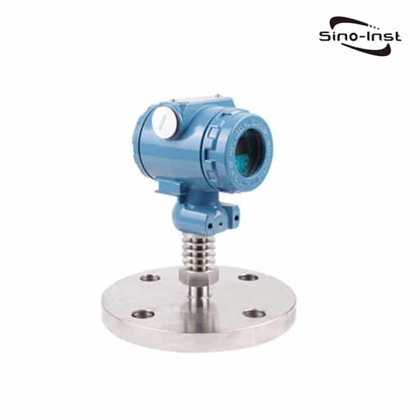
Insertion Magmeter SI-3121

Hot-tap insertion | DN80 to DN3000 | No process shutdown — for large pipes where a full-bore meter is impractical.

Stainless Steel Magmeter

SS304/SS316 body | Sanitary or industrial flange | CIP/SIP capable — food, beverage, pharma, and aggressive chemicals.

Send your pipe size, fluid, flow range, and process temperature/pressure to our engineers via the form below — we typically reply within one working day with a sized quote.

FAQ

How much straight pipe does a magnetic flow meter need?

For a single 90° elbow: 5 pipe diameters (5D) upstream and 3D downstream. Two elbows out-of-plane: 15D upstream. Valves and pumps: 20–30D upstream. Skipping straight run pulls accuracy 2–6% off, and no software fix exists.

Can a magnetic flow meter be installed vertically?

Yes — vertical with upward flow is the ideal mounting because the pipe stays full, air rises away from electrodes, and sediment passes through. Vertical with downward flow only works if the pipe stays full downstream of the meter.

Do I need grounding rings for a magnetic flow meter?

Grounding rings are required when the upstream or downstream pipe is non-conductive (PVC, FRP, lined steel) — one ring on each side. For continuous conductive metal pipe both sides, a simple bonding wire from meter housing to each pipe section is enough.

What is the minimum conductivity for a magnetic flow meter?

Most magmeters need 5 μS/cm minimum. A few high-impedance designs work down to 1 μS/cm. Magmeters do not work on hydrocarbons, distilled water, or non-polar solvents — use Coriolis or ultrasonic for those.

What flange bolt torque do I use on a magnetic flow meter?

Always follow the meter manufacturer’s torque table — values depend on liner material and gasket. As reference, Class 150 PTFE-lined meters call for 30 N·m at DN50 up to 150 N·m at DN300. Apply in three passes (30/60/100%) using a star pattern, then re-check after 24 hours.

Can I install a magnetic flow meter near a pump?

Always downstream, never upstream — pumps generate swirl that an upstream meter cannot resolve. Allow 20–30D of straight pipe between pump discharge and meter inlet. If space is tight, install a flow conditioner at the start of the run.

Request a Quote

Please enable JavaScript in your browser to submit the form

Related: straight-pipe requirements for flow meter installation.

RTD vs Thermocouple: Decision Matrix, Wiring & TCO Guide

An RTD (resistance temperature detector) measures temperature by tracking how the resistance of a platinum element rises with temperature. A thermocouple measures temperature by reading the millivolt signal produced when two dissimilar metal wires join at a hot end. Same goal, very different physics — and that difference is what makes one right for your tank, oven, or pipeline and the other a poor fit.

This guide gives you a 5-application decision matrix, the wiring rules that trip up most installers, and a 5-year cost comparison so you can make a defensible choice the next time procurement asks why you specified one over the other.

Contents

RTD and Thermocouple: Core Difference in One Sentence

An RTD changes its electrical resistance with temperature; a thermocouple generates a small voltage when its hot junction sees a different temperature than its cold junction. That single sentence drives every spec-sheet number that follows — accuracy, range, wiring complexity, drift, and cost.

The reference standards are IEC 60751 for platinum RTDs (Pt100 at 0 °C resistance of 100 Ω, α = 0.00385 Ω/Ω/°C) and IEC 60584 for thermocouples (covering Types K, J, T, N, S, R, B). Anyone selling you a sensor outside those standards is selling you trouble.

Working Principle: Resistance vs Voltage

A Pt100 RTD is a small platinum film or wire-wound coil whose resistance follows the Callendar−Van Dusen equation. Above 0 °C: R(T) = R₀[1 + AT + BT²], where R₀ = 100 Ω, A = 3.9083 × 10⁻³, B = −5.775 × 10⁻⁷. Drive a small constant current (typically 1 mA) through the platinum and you measure the resulting voltage; resistance follows by Ohm’s law.

A thermocouple is built from two dissimilar metal wires welded at one end (the measuring junction). When that junction is at a different temperature than the open end (cold junction), a millivolt-level Seebeck voltage appears. The relationship is non-linear, so the converter or transmitter uses a polynomial reference table from NIST ITS-90 to translate millivolts into temperature.

Accuracy and Stability Over Temperature

An IEC 60751 Class A Pt100 is rated to ±(0.15 + 0.002·|T|) °C. At 100 °C, that’s ±0.35 °C. A Class B Pt100 is ±(0.30 + 0.005·|T|) °C — about three times looser. RTDs drift by less than 0.05 °C per year if treated gently.

A Class 1 Type K thermocouple is rated to ±1.5 °C below 375 °C, then ±0.4% of reading above. At 1000 °C, that’s ±4 °C. Type T is the most accurate thermocouple, ±0.5 °C below 125 °C, but it only goes to 400 °C. Type S (platinum/platinum-rhodium) is more stable than K above 1000 °C but ten times the price.

Bottom line: below 600 °C, RTDs win on accuracy by a factor of five to ten. Above 600 °C, thermocouples are the only practical choice — RTDs cannot survive there long.

Temperature Range and Sensor Limits

SensorOperating RangeContinuous Use Limit
Pt100 RTD (thin film)−50 to +500 °C+400 °C
Pt100 RTD (wire-wound)−200 to +650 °C+600 °C
Type T thermocouple−200 to +400 °C+350 °C
Type J thermocouple−40 to +750 °C+700 °C
Type K thermocouple−200 to +1260 °C+1100 °C
Type N thermocouple−270 to +1300 °C+1200 °C
Type S / R / B0 to +1700 °C+1600 °C

Beyond the continuous limit, the platinum migrates in an RTD and the thermocouple wire alloys degrade. A K-type pushed past 1100 °C in air drifts at roughly 1–2 °C per 100 hours of operation. We’ve seen factory floors blame “controller drift” when the real problem was an exhausted K-type that nobody documented.

Response Time and Self-Heating

Thermocouples are faster. A 1.5 mm sheathed Type K reaches 63% of a step change in about 0.5 second in water, 5–7 seconds in air. A 6 mm sheathed Pt100 takes 3–4 seconds in water, 30+ seconds in still air. If you’re tuning a fast loop or chasing a transient, that gap matters.

RTDs also suffer self-heating: the 1 mA excitation current dissipates I²R in the element. A typical 100 Ω element with 1 mA gives 0.1 mW. In still air that’s enough to raise the reading by 0.05–0.1 °C, which is more than the Class A error budget. Thermocouples have no excitation current and no self-heating.

Wiring: 2/3/4-Wire RTD vs Type K/J/T Thermocouple

An RTD reading is just a resistance, so lead wire resistance adds directly to the measurement. A 2-wire RTD adds the full lead resistance — about 0.4 Ω per 10 m of 22 AWG copper, which is roughly 1 °C error. A 3-wire RTD subtracts one lead from the resistance bridge and cuts the lead error by about 90%. A 4-wire RTD passes current through two leads and measures voltage on the other two; lead resistance disappears from the math entirely. Use 4-wire for laboratory accuracy, 3-wire for everything else.

Thermocouples use extension wire of the same alloy as the thermocouple itself — never plain copper. Substituting copper extension on a Type K creates a second junction at the head, and that junction reads room temperature into your loop as a 4–6 °C offset. Color codes are international (IEC 60584): Type K is green positive / white negative; Type J is black/white; Type T is brown/white. For background on extension wiring conventions and shielded cables, see our note on shielded twisted-pair cables for industrial instrumentation.

For full Type K reference values, see the Type K thermocouple chart with mV reference and tolerance bands. For Pt100 element construction, see our WZP Pt100 series assembled thermal resistance page.

5-Year Cost of Ownership

Cost ItemPt100 RTD (Class A, 3-wire)Type K Thermocouple (Class 1)
Initial sensor + thermowell$140$70
Transmitter (4-20 mA)$110$95
3-wire cable (50 m)$95$210 (Type K extension)
Annual calibration (5 yrs)$60 × 5 = $300$40 × 5 = $200
Replacement during 5 yrs0 (typical)1 (high-temp service)
5-yr total$645$645 + $70 = $715

RTD wins on TCO in service below 600 °C even though the sensor itself costs twice as much. Two reasons: copper cable is much cheaper than Type K extension cable, and RTDs rarely need mid-service replacement. The math flips above 800 °C — RTDs cannot survive there, so the comparison ends.

Decision Matrix: 5 Common Industrial Applications

ApplicationTypical RangeRecommended SensorWhy
HVAC chiller water4 to 12 °CPt100 Class ATight accuracy needed for BTU calc
Boiler feedwater80 to 150 °CPt100 Class BStable, easy 3-wire run to PLC
Plastic injection mold180 to 280 °CType J or Pt100 wire-woundEither works; J is cheaper if many sensors
Heat-treat furnace700 to 1100 °CType K Class 1RTD cannot survive
Glass / kiln / cement1200 to 1600 °CType S or BOnly platinum-alloy TCs handle this

Common Selection Mistakes

  • Specifying Pt100 for a 1200 °C kiln. The platinum will diffuse into the sheath in weeks. Use Type S.
  • Running 2-wire RTD for a 30 m cable run. Lead-wire error swamps Class A accuracy. Use 3-wire minimum, 4-wire for lab work.
  • Reusing copper cable as Type K extension. You just put a 4–6 °C junction error at the head.
  • Mixing Type K and Type J how a pressure transmitter works. A Type J transmitter reading a Type K sensor under-reads by 30–40 °C at 500 °C.
  • Ignoring sheath material. Inconel 600 is fine in oxidizing air; in sulfur-bearing flue gas it pits in months. Spec Hastelloy or ceramic.

Featured Sensors from Sino-Inst

Pt100 Thermal Resistance RTD

IEC 60751 Class A | −200 to +650 °C | 2/3/4-wire — Pt100 element for HVAC, process, and lab measurement.

Industrial Thermocouple (K/J/N/T/S)

IEC 60584 Class 1 | Up to +1700 °C | Inconel / ceramic sheath — furnaces, kilns, and high-temperature process.

Universal-Input Temperature Transmitter

RTD or TC input | 4-20 mA / HART output | DIN-rail or head-mount — pairs with any sensor on this page.

Need help picking? Send your service conditions (medium, temperature range, pipe size, connection) to our engineers using the form below — we typically reply within one working day with a sized quote.

FAQ

Which is more accurate, RTD or thermocouple?

Below 600 °C, an IEC Class A Pt100 RTD beats any thermocouple by a factor of 5 to 10. Above 600 °C, RTDs degrade and thermocouples become the only practical choice.

Can I replace a thermocouple with an RTD?

Only if the service temperature stays under the RTD’s continuous limit (typically 600 °C wire-wound or 400 °C thin-film) and the transmitter accepts RTD input. You’ll also need to swap from thermocouple extension wire to plain copper.

What is the difference between Pt100 and Pt1000?

Both are platinum RTDs following IEC 60751. Pt100 has 100 Ω at 0 °C and is the industrial standard. Pt1000 has 1000 Ω at 0 °C; the higher base resistance makes lead-wire error 10x less important, so it’s popular in HVAC and 2-wire installations.

What is RTD full form?

RTD stands for Resistance Temperature Detector. It is a temperature sensor whose electrical resistance changes predictably with temperature. The most common type is the platinum Pt100 defined by IEC 60751.

Which thermocouple type should I use for general industrial work?

Type K is the default workhorse for 0–1100 °C — wide range, cheap, readily available. Use Type T if you need accuracy below 200 °C, Type J for older European installations, Type N for long-term stability above 800 °C, and Type S/R/B above 1100 °C.

How long does an RTD last in service?

Properly specified Pt100 RTDs in non-cycling service routinely last 10+ years with drift under 0.05 °C/year. Thermal cycling, vibration, and sheath corrosion shorten that life. We recommend a 12-month calibration check for any sensor in custody-transfer or food/pharma service.

Request a Quote

Please enable JavaScript in your browser to submit the form

PID Controller: Working Principle, Ziegler-Nichols Tuning & Applications

A PID controller takes the difference between where a process is and where you want it to be (the error), then computes a corrective output using three weighted terms — proportional, integral, and derivative — and feeds that output back to whatever heats, cools, opens, closes, or drives the process. The math is older than the transistor, but it still runs the world’s heat exchangers, autoclaves, motor speeds, and chemical reactors because nothing else combines its simplicity and stability.

This guide gives you the plain-English version of P, I, and D, the equation in symbols a working engineer can use, a worked Ziegler-Nichols tuning example on a temperature loop, the five mistakes that cause most tuning calls to escalate, and a spec-sheet decoder for buying a PID controller.

Contents

PID Controller Defined

A PID controller is a feedback controller that drives a process variable (temperature, pressure, flow, level, speed) toward a setpoint by adjusting one final control element (valve, heater, VFD, damper). It does this by combining three responses: a proportional response to current error, an integral response to accumulated past error, and a derivative response to predicted future error. “PID” simply names the three terms: Proportional, Integral, Derivative.

You will find PID inside dedicated panel-mount controllers, inside PLC function blocks, inside paperless recorders with control output cards, and increasingly inside the firmware of smart valves and VFDs. The physics doesn’t change with the box — only the user interface does.

What P, I, and D Each Do

Picture a tank with a heater and a thermometer, setpoint 80 °C. The thermometer reads 60 °C, so the error is 20 °C.

  • Proportional (P) reacts to the current error. Output = Kp × error. A larger Kp means a stronger heater response per degree of error. P alone leaves a permanent offset (steady-state error) because the heater turns off only when error is zero, but stops moving toward zero when there’s no error.
  • Integral (I) reacts to the sum of past errors. As long as error stays positive, the I term keeps growing, pushing the heater harder until error reaches zero. I kills the steady-state offset that P leaves behind. Too much I and the heater overshoots, then the integral has to “unwind,” causing slow oscillation.
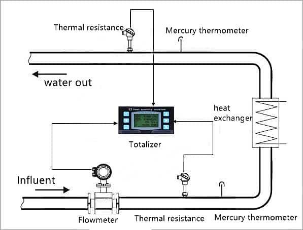
  • Derivative (D) reacts to the rate of change of error. If the temperature is rising fast, D backs off the heater early to prevent overshoot. D is a brake on aggressive P+I action. Noise on the measurement causes D to thrash, so most loops run with little or no D — temperature and slow loops use it, flow and pressure rarely do.

The PID Equation in Plain Language

The textbook form (parallel / ideal):

u(t) = Kp · e(t) + Ki · ∫ e(t) dt + Kd · de(t)/dt

where u(t) is controller output (often 0–100% to the valve or heater), e(t) is error (setpoint minus process variable), Kp is proportional gain, Ki is integral gain, and Kd is derivative gain.

Most industrial controllers use the standard ISA form instead, which is easier to tune by hand:

u(t) = Kp · [ e(t) + (1/Ti) ∫ e(t) dt + Td · de(t)/dt ]

where Ti is integral time (seconds per repeat — smaller means stronger I action) and Td is derivative time (seconds — bigger means stronger D action). When you read a controller’s display showing “PB 50%, Ti 120 s, Td 30 s,” that’s the ISA form. Proportional band PB is the inverse of Kp expressed as a percent of measurement span: PB = 100 / Kp.

Open-Loop vs Closed-Loop PID Topologies

A closed-loop PID feeds the measurement back to the controller, computes error, and drives the output. An open-loop controller just sets the output to a fixed value or follows a schedule — no feedback. Closed-loop is what people mean when they say “PID control.” Open-loop control is what runs a toaster timer.

Within closed-loop, two topologies matter: single-loop PID (one PV, one output) and cascade PID (an outer loop sets the setpoint of an inner loop). Cascade is common for heat exchangers — an outer temperature loop sets the setpoint of an inner steam-flow loop. Cascade handles disturbances 5–10x faster than a single loop.

Ziegler-Nichols Tuning: Worked Example on a Temperature Loop

Ziegler-Nichols is the most common starting point. Two methods exist: the ultimate-gain (closed-loop) method and the reaction-curve (open-loop) method. Here is the reaction-curve walk-through on a 200-L water tank heated by a 6 kW electric heater, setpoint 70 °C, current temperature 25 °C.

  • 1. Put the controller in manual. Set output to 0% and let the tank settle.
  • 2. Step the output to 50% (3 kW). Record temperature every 30 seconds.
  • 3. Plot temperature vs time. Wait until the rise straightens into a line, then plateaus at a new steady-state temperature.
  • 4. Measure: dead time L = 90 s (delay before any rise), reaction rate R = 0.20 °C/s (slope of the steep section).
  • 5. Compute K = (steady-state temp change) / (output step) = 50 °C / 50% = 1.0 °C/%.
  • 6. Apply the Z-N reaction-curve table for a PID controller: Kp = 1.2 / (R·L/K) = 1.2 / (0.20 × 90 / 1.0) = 0.067 %/°C, which is PB = 100/0.067 = 1500%… that’s clearly off for this aggressive heater.

The classic Z-N table for PID from reaction curve: Kp = 1.2 / (R·L), Ti = 2·L, Td = 0.5·L. Plugging the values: Kp = 1.2/(0.20·90) = 0.067 (output unit per °C), Ti = 180 s, Td = 45 s. In ISA terms with output in % and PV in °C, that’s about PB = 1500%, Ti = 180 s, Td = 45 s.

This is a starting point, not a finish. Z-N typically gives quarter-amplitude damping — fast response with 20–25% overshoot. For a heating loop with thermal mass, that’s often too aggressive on the I term; cut Ti in half (more I action) and increase PB (less P action) to soften the response, then re-test.

Manual Fine-Tuning When Z-N Falls Short

When Z-N gives an unstable or sluggish response, fall back to the manual procedure:

  • Set Ti = max (effectively no I) and Td = 0.
  • Increase Kp slowly. Step the setpoint up 5%. Repeat. Stop when the loop sustains an oscillation (Ku).
  • Measure the oscillation period (Tu, seconds).
  • Apply the Tyreus-Luyben softened tuning: Kp = Ku/2.2, Ti = 2.2·Tu, Td = Tu/6.3 for a PID. This gives ~10% overshoot instead of 25%.
  • If derivative makes the output thrash, set Td = 0 and accept a small overshoot — PI is often the right answer for temperature loops with noisy thermocouples.

Industrial Applications

Process TypeTypical TuningD Term Used?
Tank heating (water, slurry)PIRarely
Furnace / kilnPIDYes (slow process)
Flow loopPINo (noisy)
Pressure loop (gas)P or PINo
Level (tank w/ outflow)PNo
Motor speed (VFD)PIRarely
Autoclave / sterilizerPID with feedforwardYes

PID upgrades to model-predictive control (MPC) in large refineries and large reactors where coupled loops fight each other. For 90% of plant work, well-tuned PID still wins.

5 Common PID Tuning Mistakes

  • Tuning with the process at the wrong operating point. A loop tuned at 30% output behaves differently at 80%. Tune at the typical operating point, then test at extremes.
  • Adding derivative to a flow or pressure loop. D amplifies measurement noise into output thrash. Use PI for fast loops.
  • Forgetting integral windup. When the output saturates (valve fully open), the integral keeps accumulating. When error finally drops, the controller hangs out at full output too long. Enable anti-windup or back-calculation on every loop.
  • Tuning without bumpless transfer. Switching from manual to auto with mismatched output causes a step disturbance. Use a controller that tracks output in manual mode.
  • Confusing PB with gain. Reading “PB 100%” as “high gain” — actually means Kp = 1, which is very low. Always check whether the controller displays Kp or PB.

Selecting a PID Controller: Spec Sheet Decoder

  • Input type: Universal (TC + RTD + 4-20 mA) is worth the small price premium — one spare part fits everything.
  • Sample rate: 10 Hz minimum for temperature, 50 Hz for flow/pressure.
  • Output type: Relay (cheap, slow), SSR drive (medium-speed heater), 4-20 mA (modulating valves), or pulse (motor speed). Pick to match your final element.
  • Auto-tune: Modern controllers run a step or relay test on demand and compute initial PID values. Worth having even if you’ll fine-tune by hand.
  • Communications: RS-485 Modbus is the standard for panel-mount; HART for transmitters; EtherNet/IP or PROFINET if you’re in a PLC ecosystem. When a SCADA layer sits on top of the PLC, the controller still runs the tight loops while SCADA logs, trends, and supervises.
  • Environmental rating: IP66 for panel-front when the panel itself isn’t sealed.

If you’re integrating PID control with a recorder for trend logging and audit trails, our paperless recorders for industrial measure & control system include PID control output cards. For matching the right temperature sensor to a PID loop, see our RTD vs Thermocouple decision matrix. For signal conversion between PID outputs and 0-10 V devices, see our 4-20 mA to 0-10 V conversion guide.

Featured PID Controllers and Recorders from Sino-Inst

R7100 Paperless Recorder + PID

Universal input | Up to 16 channels | Built-in PID + auto-tune — recorder and controller in one DIN-rail unit.

R7600 Temperature Recorder

TC + RTD input | LCD trend display | Modbus RTU — for furnace, kiln, and autoclave temperature control loops.

Emerson AMS Trex Communicator

HART + FOUNDATION fieldbus | In-loop diagnostics | Bench or field — commissions PID pressure transmitter working principle and final-element devices.

Send your loop type (temperature / flow / pressure / level), I/O requirement, and ambient environment to our engineers via the form below — we typically reply within one working day with a sized quote.

FAQ

What does PID stand for?

PID stands for Proportional-Integral-Derivative, the three weighted responses a PID controller combines: P reacts to current error, I to accumulated past error, and D to predicted future error based on rate of change.

What is a PID controller used for?

PID controllers regulate one process variable — temperature, pressure, flow, level, or motor speed — by adjusting a final control element to drive the measurement toward a setpoint. Typical uses include heat exchangers, autoclaves, motor drives, gas pressure regulation, and tank-level control.

How do I tune a PID controller?

Start with auto-tune if the controller has it. Otherwise run Ziegler-Nichols: step the output and measure dead time and reaction rate, then compute Kp, Ti, Td from the Z-N table. Fine-tune by hand using Tyreus-Luyben values for less overshoot. Always tune at the typical operating point and verify at extremes.

What is the difference between P, PI, and PID control?

P alone leaves steady-state error. PI eliminates it but can overshoot. PID adds derivative to brake the response and reduce overshoot, at the cost of noise amplification. Use P for level, PI for flow/pressure, PID for temperature and slow processes.

What is proportional band (PB) in a PID controller?

Proportional band is the inverse of proportional gain expressed as a percent of measurement span: PB = 100 / Kp. A PB of 100% means the controller swings from 0% to 100% output across the full measurement range. Smaller PB means more aggressive response.

Why is integral windup a problem?

When the controller output saturates (valve fully open or closed), the integral keeps accumulating error even though more output isn’t available. When error finally drops, the integral has to “unwind” before the controller backs off, causing severe overshoot. Anti-windup logic or back-calculation prevents this.

Where is PID control still used today?

PID still runs the majority of regulatory control in chemical plants, power stations, food and pharma manufacturing, water treatment, HVAC, and motor drives. Model-predictive control replaces PID at the supervisory level in large coupled systems, but underneath the MPC layer the field loops are almost always PID.

Request a Quote

Please enable JavaScript in your browser to submit the form