Shaft Torque Sensor: Working Principle, 3 Coupling Architectures, Spec Sheet, Diagnostics

Updated 2026-05-11 by the Sino-Inst engineering team.

A shaft torque sensor sits between a motor and the load and reads the twisting force on the rotating shaft. The output is a 4-20 mA, frequency, CAN, or RS485 signal that a test bench, dynamometer, or process controller logs in real time. Most field failures on these instruments are not the sensor itself — they are misalignment, vibration coupling from the pump or motor, or a coupling that was the wrong choice for the speed and torque envelope.

This guide covers what a shaft torque sensor measures, the three working principles (strain gauge, SAW, magnetoelastic), the three mechanical coupling architectures you have to choose between, how to read a spec sheet, the three dominant failure modes, a 5-step diagnostic checklist, maintenance intervals by signal-coupling type, and the decision tree for re-zero / re-cal / replace.

Contents

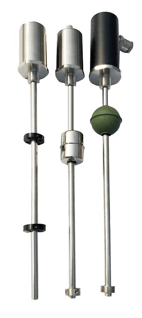
Shaft torque sensor in drivetrain test bench

Shaft Torque Sensor Definition and Role in the Drivetrain

A shaft torque sensor — also called a rotary torque transducer or in-line torque sensor — measures the torsional moment T (in N·m or lbf·ft) that one side of the drivetrain delivers to the other while the shaft is turning at speed n. Inserted between the prime mover and the load, it sees real-time torque without disturbing the rotational coupling. The output reports both static torque (when the bench is locked) and dynamic torque (during transient acceleration, gear-shift, or stall).

The sensor’s job is to convert a mechanical twist into a clean electrical signal that survives slip rings, brush wear, or non-contact telemetry over the life of the test stand. For the broader concept of how torque transducers fit into instrumentation, see our torque transducer overview.

Working Principle: Strain Gauge, SAW, and Magnetoelastic

Three sensing technologies dominate shaft torque measurement. They differ by 10× in price, by signal coupling, and by what they tolerate at speed.

  • Strain gauge. Four resistive gauges bonded to the shaft in a Wheatstone bridge sense the surface strain caused by the torsional shear. Accuracy ±0.1 % FS, range 0.1 N·m to 100 kN·m. The signal must leave the rotating shaft via slip rings, brushless rotary transformer, or digital telemetry — that signal-coupling choice drives maintenance.
  • Surface Acoustic Wave (SAW). Piezoelectric resonators on the shaft surface shift frequency under stress. The signal is read non-contact via an RF antenna. No moving wires, no brushes, no slip-ring wear; accuracy ±0.5 % FS, range 1 N·m to 5 kN·m. Wider temperature window than strain gauge but more sensitive to electromagnetic interference.
  • Magnetoelastic. A ferromagnetic shaft region is magnetised; torsional stress changes its permeability, which a pickup coil reads. Non-contact, rugged, but accuracy is ±1 % FS at best. Used in automotive electric power steering (EPS) and high-throughput production lines where ±1 % is enough.

Three Mechanical Coupling Architectures: Inline, Flange, and Rotor-Stator

Once the sensing technology is fixed, the mechanical architecture decides how the sensor mounts in the drivetrain.

ArchitectureSpeed limitBest forTrade-off
Inline shaft-to-shaft15,000-30,000 rpmDyno test cells, gearbox R&DNeeds precise alignment; flex couplings essential
Flange-to-flange5,000-10,000 rpmMarine, wind turbine, large industrial drivesHeavy; pricey for low torque
Rotor-stator (split, non-contact)20,000+ rpmRetrofit on existing shafts, EPS, surface telemetryAir gap and runout matter; calibration is more complex

Pick inline for new builds where the test bench is being designed around the sensor. Pick flange-to-flange for big drives where the shaft is too large to interrupt. Pick rotor-stator when you cannot break the shaft and just need to clamp a stator around a magnetised section. For the broader test-bench torque measurement context, see our stationary vs rotary torque sensors guide.

Measurement Range, Accuracy, and the Spec Sheet Decoded

Five spec-sheet fields decide whether a shaft torque sensor fits the loop:

  1. Nominal torque (T_nom) and overload limit. Spec the sensor for 1.3-1.5 × your worst-case dynamic peak, not your steady-state. An overload limit of 200 % of T_nom is the industry standard but check the catalog — some economy units stop at 130 %.
  2. Accuracy class. ±0.05 % FS is custody-grade. ±0.2 % FS is standard for dyno work. ±1 % FS is production-line acceptable. Read whether the figure is “linearity” alone or “linearity + hysteresis + repeatability combined” — the latter is the honest one.
  3. Speed rating and bandwidth. Maximum continuous rpm and signal bandwidth (Hz). A bandwidth lower than 2× your shaft frequency aliases — at 3000 rpm = 50 Hz fundamental, you need at least 100 Hz bandwidth to catch the twist signature.
  4. Signal coupling and output. Slip ring, rotary transformer, RF telemetry, or SAW interrogation. Output: ±10 V analogue, 4-20 mA, frequency (PWM), or digital (CAN/Modbus/Profinet).
  5. Environment. Operating temperature, IP rating, vibration class, and EMC compliance. A test cell next to a 200 kW VFD will spray broadband noise; pick a sensor with explicit EMC class B compliance and shielded cabling.

The calibration certificate that ships with the sensor is your traceability proof. For the calibration practices that keep the certificate meaningful between annual recals, see our note on how to calibrate field instruments — the principles transfer directly.

Three Dominant Failure Modes and What They Look Like on the Trace

Failure modeSymptom on the traceRoot causeRecoverable?
Zero driftStatic reading creeps away from 0 over hoursStrain gauge adhesive aging, slip-ring contact resistance, temperature gradient on the bodyYes — re-zero, then re-cal if it returns
Span lossSensor reads only 80-90 % of the dyno’s calibrated torqueCracked gauge bond, partial slip-ring brush wear, SAW antenna detuning from cable shiftSometimes — recal often masks the underlying damage
Noise / oscillation30-200 Hz pickup on the trace, no actual torque changeVibration coupling from upstream pump or motor; ground-loop noise in the signal cableYes — isolate or move the cable
Catastrophic breakReading flatlines or saturates to ±FSOverload event, fatigue crack through gauge, shaft seizureNo — sensor is end-of-life

5-Step Diagnostic Checklist When Readings Look Wrong

  1. Re-zero at no-load. Disengage the load, let the shaft turn at idle for 60 seconds, command a zero. If the trace returns to 0.000 N·m and stays there for 5 minutes, the offset is just thermal drift — not a fault.
  2. Shunt-cal check. Push the shunt-cal button or send the shunt-cal command. The sensor should output its rated shunt value within ±0.5 %. If it does not, the span path (bridge resistance, signal-conditioner gain) is degraded.
  3. Two consecutive run-ups. Run the dyno to nominal torque twice in succession. If the second run reads more than 0.2 % FS different from the first, you have hysteresis from a sticky coupling or a strain-gauge crack.
  4. Alignment and runout check. Dial-indicate the input and output shafts at the coupling. More than 0.05 mm TIR loads the sensor body with bending moments that read as false torque.
  5. Cross-check with motor electrical torque. A modern VFD reports motor torque from current and rotor angle to ±5 %. If the dyno torque sensor diverges from the VFD-derived torque by more than 5 % across the speed range, suspect the sensor, not the motor.

Maintenance Intervals by Signal-Coupling Type

  • Slip-ring + brush coupling: Inspect brushes every 2000 operating hours; replace at 5000 hours or 25 % brush remaining. Clean slip ring with isopropyl alcohol monthly. Recal annually.
  • Rotary-transformer (brushless) coupling: Inspect every 8000 hours; no consumable parts. Recal every 18-24 months unless mounted in harsh vibration.
  • RF telemetry coupling: Battery or inductively powered. Battery-powered units need pack replacement at 2-3 years. Antenna alignment check yearly. Recal every 24 months.
  • SAW (non-contact, no power on rotor): No rotor maintenance. Stator antenna realign every 12 months or after any motor swap. Recal every 24-36 months — drift is mostly in the interrogator electronics, not on the rotor.

For the broader installation hygiene that applies to any rotating-shaft instrument — vibration isolation, cable routing, EMC — see our pressure transmitter installation guide. The signal-conditioner mounting principles transfer directly.

When to Re-Zero, When to Re-Cal, When to Replace

  1. Re-zero when the offset is less than 0.5 % FS and stable after a 60-second idle. Operators can do this themselves. Trend the offset week-on-week; growing drift is the early signal of a slip-ring or adhesive problem.
  2. Re-cal when the offset is between 0.5 % and 2 % FS, or when shunt-cal disagrees with the certificate by more than 0.5 %. Requires a calibration arm and traceable weights, typically a service-house job.
  3. Replace when the sensor saturates, when two run-ups disagree by more than 1 % FS at nominal torque, when shunt-cal fails completely, or when the unit has seen an overload above 150 % T_nom. Once the strain bond or SAW resonator is cracked, recal cannot restore traceability.

Featured Shaft Torque Sensors

807 Rotary Torque Sensor (15,000 rpm)

Inline strain-gauge, ±0.1 % FS, rotary-transformer signal coupling, ±10 V / 4-20 mA / frequency output.

120 Reaction Torque Sensor

Static torque wrench / motor / engine test, ±0.5 % FS, 0-1000 N·m, 4-20 mA + Modbus.

56 Micro Reaction Torque Sensor

Small-torque bench, ±0.2 % FS, 0-10 N·m, low-noise strain-gauge bridge.

FAQ

How does a shaft torque sensor work?

Three principles dominate: strain gauges in a Wheatstone bridge sense torsional surface strain; SAW resonators shift frequency under torque; magnetoelastic sensors detect permeability changes in a magnetised shaft region. The signal leaves the rotating element via slip rings, rotary transformer, RF telemetry, or non-contact SAW interrogation.

What is a shaft torque sensor?

A rotary torque transducer inserted in a drivetrain that measures the torque transmitted through the shaft while it is turning. Output is ±10 V, 4-20 mA, frequency, or digital (CAN/Modbus).

What is shaft torque?

The torsional moment T = F·r transmitted around the axis of a rotating shaft, measured in N·m (SI) or lbf·ft (US). Power transmitted is P = T × ω, where ω is angular velocity in rad/s.

What is the difference between an industrial shaft torque sensor and an automotive steering shaft torque sensor?

Industrial sensors are precision test instruments — ±0.1 to 0.5 % FS, recalibrated annually, used on dynos and R&D benches. Automotive EPS sensors are embedded in the steering column to feed the electric power steering ECU. They are typically magnetoelastic, ±1-2 % FS, and not designed for traceable measurement.

How is a shaft torque sensor installed?

Insert between input and output shafts using flexible couplings on both sides to absorb alignment error. Keep the input-output runout under 0.05 mm TIR. Route signal cable away from motor power leads, and ground at the conditioner end only to avoid ground loops.

What measurement range does a shaft torque sensor cover?

Strain-gauge sensors span 0.01 N·m (micro reaction) to 100 kN·m (marine drive). SAW typically 1 N·m to 5 kN·m. Spec the nominal torque at 1.3-1.5 × your worst-case peak, not your steady-state.

How often should a shaft torque sensor be calibrated?

Annually for slip-ring units, every 18-24 months for rotary-transformer and RF telemetry, every 24-36 months for SAW. Always recal after any overload event above 150 % nominal torque.

Need help picking a shaft torque sensor for your test bench or drive? Our engineers can quote and ship within 24 hours — message us with peak torque, shaft speed, accuracy band, and signal-coupling preference.

Request a Quote

Request a Quote

Please enable JavaScript in your browser to submit the form

Density Meter: Working Principle, 6 Technologies, Spec Sheet, Compensation, Calibration

Updated 2026-05-11 by the Sino-Inst engineering team.

A density meter measures the mass per unit volume of a liquid, slurry, or gas, usually in real time and at process pressure. The reading is what you bill on, what you blend by, and what tells custody-transfer custody that you handed over the product you said you would. The same number — “density” — can be measured six different ways, and the wrong technology for the wrong service makes a 0.1 % error look like 5 %.

This guide covers what a density meter does, the working principle behind each sensing technology, a side-by-side comparison of the six main types, how to pick by fluid, how to read a spec sheet, temperature and pressure compensation, calibration, and four install pitfalls that wreck field accuracy.

Contents

Density Meter Definition and Industrial Role

A density meter reports the density (ρ, in kg/m³ or g/cm³) of a fluid in real time. Density is mass divided by volume, but in process plants it doubles as a stand-in for concentration, dilution, fermentation progress, hydrocarbon API gravity, brine strength, or polymer solids content. A 0.5 % shift in density at the right point in a process tells the operator that a steam coil has stuck open, that a feed tank is being diluted by rinse water, or that a custody-transfer batch is off-spec — long before any other parameter catches it.

For background on the SI and field units density meters report — kg/m³, g/cm³, API gravity, °Brix, °Baumé — see our note on the unit of measurement for density.

Working Principle of a Density Meter

Every density meter exploits one of four physical effects: mechanical resonance shift, gravitational hydrostatic pressure, acoustic time-of-flight, or nuclear absorption. The choice of effect drives accuracy, fluid compatibility, and price.

  • Mechanical resonance. A tube or fork is vibrated at its natural frequency. As denser fluid loads the structure, the resonant frequency drops. Coriolis tubes, tuning forks, and Anton-Paar-style U-tubes all use this principle. Resolution is excellent (4-decimal density), but the cell sees the process directly and must tolerate it.
  • Hydrostatic ΔP. Two pressure transmitters at known elevations in a tank read the column weight; density is ΔP / (g·h). Slow, cheap, and immune to fluid type, but tank-mounted only and accuracy is limited by the transmitters.
  • Acoustic time-of-flight. A pulse is launched across the fluid; the speed of sound depends on density and bulk modulus. Non-intrusive (clamp-on), but fluid-of-known-composition only.
  • Gamma absorption. A small radioactive source on one side of the pipe, a detector on the other. Beam attenuation tracks density. Works on slurries, opaque flows, and high-pressure service where nothing else survives, but needs a radiation safety case.

Six Density Meter Technologies, Side by Side

Six technologies dominate field and lab density measurement. They span 5 decades of accuracy and 3 decades of price.

TechnologyAccuracy (kg/m³)Best forAvoid forCost band
Coriolis mass flow + density±0.5Custody transfer, hydrocarbons, dosingSlurries with gas voids, very low flow$$$$
Tuning fork (insertion or in-line)±1Tank-side concentration, refining, foodFibrous solids that snag the fork$$
Oscillating U-tube (lab/portable)±0.01Lab reference, batch QC, °Brix labsIn-line service, opaque slurries$$$
Differential pressure (hydrostatic)±2-5Open tanks, settling slurriesClosed pressure vessels, fast process$
Ultrasonic time-of-flight±2Non-intrusive retrofits, clean fluidsGassy or particulate-laden streams$$
Gamma (nuclear) densitometer±1-5Drilling muds, ore slurries, coke, opaque high-PAnywhere licensing is a problem$$$$

Coriolis is the de-facto custody-transfer instrument for hydrocarbons because it gives mass flow and density simultaneously at ±0.1 % MV — but it cannot tolerate the gas voids that drilling mud delivers daily. For that, gamma is the answer. Oscillating U-tube wins the lab and the portable spot-check role; it is the reference for °Brix, °Baumé, and API gravity. For a deeper look at how Coriolis derives density from its tube resonance, see our Coriolis density measurement guide.

Process-Specific Density Meter Selection by Fluid Type

The fluid dictates the technology more than the budget does. A picker by service:

  • Crude oil and refined hydrocarbons: Coriolis for custody transfer, oscillating U-tube for assay lab. See our density of crude oil guide for API gravity and ASTM D1250 corrections.
  • Sugar, °Brix, fermentation: Oscillating U-tube for lab, tuning fork in-line for blending tanks.
  • Acid (H₂SO₄, HCl, HNO₃): Tuning fork in tantalum or PEEK wetted parts, or non-intrusive ultrasonic.
  • Settling slurries and drilling muds: Gamma densitometer — survives abrasion that destroys vibrating cells. For more on slurry behaviour, see our industrial slurry density measurement note.
  • Polymer melts and high-viscosity fluids: Coriolis or hydrostatic ΔP; avoid tuning fork (high damping kills resolution).
  • Cryogenic LNG and LPG: Coriolis with cryogenic-rated tubes — also the standard custody-transfer choice on LNG terminals.

Density Meter Spec Sheet Decoded

A density meter spec sheet drowns the buyer in numbers. Five fields decide whether the instrument fits the loop:

  1. Reference temperature. Density is meaningless without it. ASTM uses 15 °C, API uses 60 °F, food uses 20 °C. A “1000 kg/m³ water” reading at 4 °C is not the same as at 20 °C — there is a 0.18 % swing in between.
  2. Accuracy band (specified vs typical). Anton-Paar publishes ±0.0001 g/cm³ for the lab U-tube but only at 20 °C and after a 30-minute warm-up. Process Coriolis is ±0.5 kg/m³ across the full operating envelope. Compare like-for-like.
  3. Span vs zero stability. Span drift moves the calibration slope; zero drift moves the intercept. A spec sheet that quotes only “accuracy” without splitting the two is hiding something.
  4. Process connection and wetted materials. 316L is default; tantalum, Hastelloy C276, and PTFE-lined are extra-cost. Get the material right and the meter lasts; get it wrong and you lose it to corrosion in months.
  5. Output and protocol. 4-20 mA + HART, Modbus RTU, Foundation Fieldbus, EtherNet/IP. Match the loop, not the brochure.

Temperature and Pressure Compensation for Field Accuracy

Fluid density changes about 0.1 % per °C and about 0.005 % per bar. Without compensation a Coriolis or tuning fork running at 60 °C and 20 bar will read 5-6 kg/m³ off its 20 °C / 1 bar factory calibration. Modern transmitters apply two corrections automatically:

  • Temperature compensation. An RTD glued to the resonating element or the U-tube reads element temperature and applies the manufacturer’s temperature coefficient.
  • Pressure compensation. A static-pressure input (4-20 mA from a separate transmitter, or HART-burst from the same loop) corrects the resonator stiffness shift with line pressure.

Two field traps: first, the temperature sensor reads the wall of the cell, not the fluid bulk — a fast process step (a steam injection, a cold-water rinse) gives a transient density error until the wall equilibrates. Second, the pressure correction needs the actual line pressure, not the design pressure; a stuck pressure transmitter feeding a constant 16 bar will drift the density reading whenever the line moves up to 25 bar.

Calibration Procedure and Drift Management

Density meter calibration is a two-fluid procedure, regardless of technology:

  1. Air (or N₂) zero. Drain and dry the cell, take a reading at atmospheric pressure and known temperature. Compare to tabulated air/N₂ density at that T,P.
  2. Reference fluid span. Fill the cell with degassed deionised water (or another traceable reference). Read at known T,P, compare to tabulated value (999.0 kg/m³ at 15 °C, 998.2 at 20 °C).
  3. Adjust offset and slope. Most transmitters expose a two-point cal interface; enter the air and water readings, the firmware computes the new offset and slope.
  4. Verify with a third fluid. Run a second reference (denser organic solvent like trichloroethylene at 1462 kg/m³, or a sodium-chloride brine) and check the meter is within ±0.5 kg/m³ of the tabulated value.

Field intervals: lab U-tubes monthly, Coriolis and tuning fork annually, gamma every two years (with a source-decay correction built into the firmware). Drift rates: 1-2 kg/m³ per year for Coriolis and tuning fork on clean fluids, faster on abrasives. If the meter swings more than 0.5 % between cal cycles, look at coating, erosion, or mounting strain before declaring the sensor faulty.

Four Install Pitfalls That Ruin Field Accuracy

  1. Strain from pipe expansion. A Coriolis or tuning fork bolted between rigid supports picks up axial stress as the line heats up; the resonator stiffens and the density reading drifts low by 5-10 kg/m³. Use a flexible mount or a thermal-expansion loop upstream.
  2. Gas entrainment. A single 1 mm bubble at 10 barg can pull a Coriolis reading 20 kg/m³ low for several seconds. Mount horizontally with the tubes upwards, or install a gas eliminator if the line is suspect.
  3. Wrong orientation for tank settling. Tuning fork insertion probes mounted at the bottom of a tank read the heavy phase, not the bulk. Mount at the mid-tank or in the recirculation loop.
  4. Vibration coupling from pumps. A positive-displacement pump 2 m upstream of a Coriolis at 10-15 Hz couples into the resonator and adds 1-2 kg/m³ noise. Decouple with a flexible connector or move the meter further away. For more on equivalent piping discipline, see our industrial applications of density meters note.

Featured Density Meters

Online Density Meters by Differential Pressure

Tank-mount ΔP density, 0-3000 kg/m³, 4-20 mA + HART, ±2 kg/m³ accuracy.

Portable Density Meter (Tuning Fork)

Hand-held tuning fork, 0-3000 kg/m³, °Brix / °API conversion, data-log.

In-line Tuning Fork Density Meter

In-line insertion fork, 0-2000 kg/m³, 4-20 mA + Modbus, ±1 kg/m³ accuracy.

FAQ

What is a density meter?

An instrument that measures the mass per unit volume (density) of a fluid at process conditions. Real-time units are typically kg/m³ or g/cm³; derived units include °Brix, °Baumé, and API gravity.

How does a density meter work?

The four working principles in use are mechanical resonance shift (Coriolis, tuning fork, U-tube), hydrostatic ΔP, acoustic time-of-flight, and nuclear absorption. Each maps a physical effect that depends on density into an electrical signal.

What does SG 20/20 mean?

Specific gravity 20/20 means the density of the sample at 20 °C divided by the density of pure water at 20 °C. It is dimensionless and slightly different from SG 60/60 (the API petroleum convention at 60 °F).

Can density be measured in g/m³?

Technically yes, but no one does for liquids — values would run into millions. Liquids use kg/m³ or g/cm³; only very low-density gases (atmospheric particulate, trace contaminants) are reported in g/m³.

How do you read a density meter?

Read the primary display (kg/m³ or g/cm³), then check the reference temperature it is corrected to. If the reading is at process temperature uncorrected, apply the manufacturer’s T-coefficient to get the value at 15 °C or 20 °C reference.

How often should a density meter be calibrated?

Lab oscillating U-tubes monthly. Process Coriolis and tuning fork annually. Gamma densitometers every two years with source-decay correction. Verify after any major piping work that could induce strain.

Which density meter is best for slurries?

Gamma densitometer for abrasive or opaque slurries (drilling muds, ore concentrates). For lighter slurries with gas tolerance, a properly-mounted Coriolis can work. Avoid tuning fork in fibrous slurries.

Need help picking a density meter for your fluid, accuracy band, and budget? Our engineers can quote and ship within 24 hours — message us with the service, line pressure, fluid composition, and target accuracy.

Request a Quote

Request a Quote

Please enable JavaScript in your browser to submit the form

Dew Point Meter for Compressed Air: PDP, ISO 8573-1, Sensors, and Out-of-Spec Fix

Updated 2026-05-11 by the Sino-Inst engineering team.

A dew point meter for compressed air reports the pressure dew point (PDP) — the temperature at which water vapour condenses out of the air at line pressure. That single number decides whether your dryer is delivering the ISO 8573-1 humidity class your plant signed up for. Most field problems with moisture in compressed air are not dryer failures; they are wrong sensor selection, wrong placement, or a sensor that has drifted 8 °C since the last calibration.

This guide covers PDP fundamentals, the ISO 8573-1 classes that fix sensor range, three sensor technologies (chilled mirror, aluminum oxide, capacitive polymer), a step-by-step measurement procedure for in-line and portable instruments, dryer pairing, what to do when the reading is out of spec, and the four mistakes that pull readings off year after year.

Contents

Pressure Dew Point Explained for Compressed Air

Pressure dew point is measured at the working pressure of the line. Atmospheric dew point is the same temperature after the sample has been expanded back to 1 atm. The two numbers are not interchangeable. A sample at 7 barg with +3 °C PDP is equivalent to roughly -23 °C atmospheric dew point — a 26 °C gap that catches engineers out on audits.

This matters on every spec sheet. Compressed air specifications are written in PDP, but most cheap psychrometers report atmospheric dew point. Take a hand-held instrument, vent the sample to ambient, and read -23 °C — you have not exceeded ISO 8573-1 Class 4 (+3 °C PDP), you have just barely met it. Reading the wrong column has flunked more compressed-air audits than any real dryer fault. Always confirm whether a number is at line pressure or after expansion.

The conversion isn’t intuitive either. At 10 barg the gap widens further, so a portable meter reading -30 °C after expansion does not mean you have Class 2 air. For background on absolute vs gauge pressure references, see our static vs dynamic pressure guide.

ISO 8573-1 Humidity Classes and Sensor Range Selection

ISO 8573-1:2010 defines seven humidity classes. The class you have to meet is set by what the air feeds, not by the dryer you happen to own. Pick the class first; the sensor range falls out of it.

ClassPDP targetTypical useSensor range needed
1≤ -70 °CPharma, semiconductor, breathing air-100 to -40 °C
2≤ -40 °CInstrument air, paint spray, food packaging-80 to -20 °C
3≤ -20 °CPlant control air in cold climates-60 to 0 °C
4≤ +3 °CGeneral plant air, pneumatic tools-20 to +20 °C
5≤ +7 °CLight pneumatic load (refrigerant dryer)-10 to +20 °C
6≤ +10 °CCoarse air, agitation0 to +30 °C
XUser-definedProcess-specificBy spec

One trap to watch: a Class 2 sensor (-80 to -20 °C) loses resolution above -20 °C, so it cannot tell you whether you have exceeded Class 4. Spec to your worst-case PDP target plus about 20 °C of headroom, not your best-case. A second trap: 4-20 mA outputs are usually scaled across the full sensor span, so if you buy a -80 to +20 °C sensor and only care about Class 4 territory, you waste 75 % of the resolution on the lower end. Either scale the transmitter output to your range of interest, or buy a Class-matched sensor.

Three Sensor Technologies: Chilled Mirror, Al₂O₃, and Capacitive Polymer

Three technologies dominate field dew point measurement in compressed air. They differ by 5–10 °C in absolute accuracy and by an order of magnitude in price and maintenance.

TechnologyRangeAccuracyBest forCost band
Chilled mirror-90 to +90 °C±0.1 °CLab reference, cal standard$$$$
Aluminum oxide capacitive (Al₂O₃)-110 to +20 °C±2 °CCryogenic, Class 1, hydrogen service$$$
Capacitive polymer film-80 to +60 °C±2 °CClass 2-4 plant air, instrument air$

Chilled mirror is the laboratory primary — a cooled metal mirror with optical detection of condensation. The reading is by definition correct because it physically forms condensate at the dew point. Slow (minutes per reading) and expensive, and the mirror needs cleaning. Use it as your calibration reference, not as the in-line sensor.

Aluminum oxide capacitive sensors use a porous Al₂O₃ layer whose dielectric constant changes with adsorbed water. They tolerate extreme dryness (-110 °C is realistic), which makes them the choice for hydrogen, cryogenic nitrogen, and Class 1 pharma air. Drift is moderate at 3-5 °C per year, and the cell needs an annual factory bake-out.

Capacitive polymer film sensors are the workhorse for compressed air in the Class 2-4 range. They are faster (90 % response in 30-60 seconds with proper sampling), cheaper, and have a 200 °C auto-bake cycle that drives moisture back out daily. Drift is 2-3 °C per year in clean air but climbs to 5-10 °C in oily lines, which is why filtration matters more than the sensor brand.

Dryer Technology and Achievable Pressure Dew Point

The dryer fixes the floor your sensor will see; pick the right pair so the sensor sits in the middle of its calibrated range.

  • Refrigerant dryer: +3 to +10 °C PDP. Cheapest, used for Class 4-6.
  • Heatless desiccant dryer: -40 °C PDP nominal, -70 °C achievable. Class 2 standard, Class 1 with tight tower switching.
  • Heated desiccant dryer: -40 to -70 °C PDP, lower purge loss than heatless (5-7 % vs 14 %).
  • Membrane dryer: -20 to -40 °C PDP for low-flow point-of-use applications.

If your specification calls for Class 2 air but you own a refrigerant dryer, no amount of sensor calibration fixes that — you need a desiccant tower. The dew point meter is a diagnostic tool, not a corrective one. For broader gas-dew-point context (CO₂, N₂, hydrocarbons), see our guide to what gases a dew point meter can detect.

Step-by-Step Procedure to Measure Dew Point in Compressed Air

There are two field procedures, depending on whether you have an in-line transmitter or a portable spot-check meter.

In-line transmitter (continuous monitoring):

  1. Confirm the sensor is mounted downstream of the dryer outlet and downstream of the coalescing filter, but upstream of any after-filter that could retain moisture.
  2. Open the sample bleed valve to 1-2 NL/min purge through the measuring chamber. Without purge, response time stretches from minutes to hours.
  3. Let the 4-20 mA / RS485 output settle for 5-15 minutes after any pressure or flow change. Capacitive polymer sensors respond fast, but gas exchange around the film is the rate-limiter.
  4. Trend continuously over 24 h. A clean compressed air line should show diurnal swing under 3 °C; larger swings point at dryer cycling problems.

Portable spot-check (audit):

  1. Connect the portable meter to a Minimess test point downstream of the dryer using a 2-3 m sample hose in stainless or PTFE. Avoid rubber — plasticisers outgas into the sensor and shift the calibration warm.
  2. Set the flow regulator on the meter to 1 NL/min. Vent any condensate trap before starting.
  3. Allow 15-30 minutes for the reading to stabilise. Keep the sample at line pressure during the wait — measuring at a vented sample reads atmospheric dew point, not PDP.
  4. Record both PDP and line pressure on the audit log. The two together let you compute atmospheric dew point and cross-check any downstream spec written in that reference.

The same straight-run logic that shapes flow-meter sample placement applies here — see our upstream and downstream straight pipe guide for the underlying sampling principle.

Sensor Placement and Sample Conditioning

Install the in-line probe at least 2 metres downstream of the dryer outlet, after the coalescing filter, and before the final after-filter. Three placement rules from field installations:

  1. Mount the probe horizontally, never sensor-down. Liquid water collecting on the polymer destroys the calibration in hours.
  2. Use stainless or PTFE in the sample line. PVC and rubber outgas plasticisers that load the sensor.
  3. Keep the sample line under 5 m. Long lines act as moisture buffers and slow the reading by an hour or more.

Sample conditioning is where most field measurements quietly fail. A common mistake is plumbing the probe straight into the dryer header without a sample loop — at zero flow, the polymer equilibrates to whatever the dead leg has been doing for the past week, not to the live process. A 1-2 NL/min bleed is the cheapest insurance against this.

How to Reduce Pressure Dew Point When You Are Out of Spec

If the dew point meter shows you above your ISO 8573-1 target, work down this list before assuming the dryer has failed.

  1. Verify the reading. Confirm the sensor was calibrated in the last 12 months. A polymer sensor running 8 °C high after a year in oily air is normal, not faulty.
  2. Check the pre-filter. Liquid water carryover from the receiver overwhelms any dryer downstream. Replace coalescing elements at 4000 hours or per ΔP alarm.
  3. Inspect dryer cycling. On twin-tower desiccant dryers, a stuck purge valve or failed tower switch raises PDP by 10-30 °C. Listen for the tower changeover at the timer interval.
  4. Check ambient and inlet conditions. Refrigerant dryers degrade above 35 °C inlet temperature. Heatless desiccant dryers consume up to 14 % of throughput as purge — under-sizing the dryer for plant air demand shows up as PDP creep.
  5. Upgrade dryer technology. Refrigerant only reaches +3 °C PDP. If the spec calls for Class 2 or better, you need a desiccant tower added in series or in replacement. For installations facing pressure-side fluctuations alongside moisture, our pressure transmitter installation guide covers the same impulse-line discipline.

Calibration and Drift: Why a 1-Year-Old Sensor Reads 8 °C High

Polymer-capacitive dew point sensors drift by 2-3 °C per year in clean air and 5-10 °C in oily air. Four practical errors accelerate that:

  1. Skipping the coalescing filter. Compressor oil mist coats the polymer and shifts the calibration warm — typically 5-8 °C in 12 months.
  2. Wet exposure. A single bulk-water hit damages the dielectric layer permanently. Once a polymer sensor has seen liquid water, it never reads correctly again.
  3. Neglected auto-cal cycles. Modern sensors run a 200 °C bake every 24 h to drive moisture out; if power is interrupted, drift compounds month over month.
  4. Annual factory cal that ignores process conditions. A sensor returned for cal at -40 °C reference will not match a +3 °C process. Calibrate at the band you actually run in.

Featured Dew Point Meters for Compressed Air

Dew Point Transmitter 608 Series

In-line probe, -80 to +20 °C PDP, 4-20 mA / RS485 Modbus, ±2 °C accuracy.

Dew Point Meter 602 Series

Wall-mount display, -60 to +60 °C PDP, alarm relays, 35 bar service.

Portable Dew Point Meter

Hand-held audit tool, integrated sample cell, -50 to +20 °C PDP, data-log.

FAQ

How do you measure the dew point of compressed air?

Use a polymer-capacitive sensor in a sample cell at line pressure with 1-2 NL/min purge through the cell. Allow 5-15 minutes for in-line transmitters and 15-30 minutes for portable spot-checks to settle on each new reading.

What is the dew point limit for compressed air?

It depends on the ISO 8573-1 class required. Instrument air is usually Class 2 at -40 °C PDP; general plant air is Class 4 at +3 °C PDP; pharma and semiconductor air is Class 1 at -70 °C PDP. There is no single number.

How do you reduce the dew point in compressed air?

Verify sensor calibration first, then check coalescing filter ΔP, then check dryer cycling and ambient inlet temperature. If readings are confirmed and the dryer is healthy, the only durable fix is upgrading from refrigerant to desiccant drying, or adding a desiccant tower in series.

What is the difference between pressure dew point and atmospheric dew point?

Pressure dew point is measured at line pressure; atmospheric dew point after expansion to 1 atm. 7 barg air at +3 °C PDP corresponds to roughly -23 °C atmospheric dew point — the two are not interchangeable on a spec sheet.

What is the best dew point for instrument air?

ISA-7.0.01 calls for instrument air at least 10 °C below the lowest ambient temperature the air will see. In temperate plants that means -40 °C PDP (Class 2); in arctic service, -70 °C PDP (Class 1).

How often should a compressed air dew point sensor be calibrated?

Annually for clean instrument air, every 6 months for plant air on oil-lubricated compressors. Send the sensor back at the PDP band you actually operate in, not the factory default.

Can a dew point meter be installed downstream of an oil filter?

Yes — and it should be. Place the probe after the coalescing oil filter but before the after-filter. Oil mist on the polymer is the fastest way to ruin the sensor.

Which sensor technology is best for Class 1 compressed air?

Aluminum oxide capacitive sensors reach -110 °C and are the right choice for Class 1 air (-70 °C PDP). Capacitive polymer sensors lose resolution below -60 °C and should not be used for pharma or semiconductor service.

Need help picking a dew point meter for your dryer and ISO 8573-1 class? Our engineers can quote and ship within 24 hours — message us with your line pressure, target PDP, and flow rate.

Request a Quote

Request a Quote

Please enable JavaScript in your browser to submit the form

Torque Transducer Selection: Reaction vs Rotary, Slip Ring vs Telemetry, and Accuracy Class

Updated: May 10, 2026 — by Sino-Inst Engineering Team

For shaft-mounted sensing on rotating drivetrains — strain gauge, SAW, magnetoelastic, and the maintenance/diagnostic playbook — see our shaft torque sensor guide.

A torque transducer turns mechanical torque on a shaft or flange into a calibrated electrical signal — usually 4-20 mA, 0–10 V, or a digital frame. The wrong choice is expensive: a reaction sensor on a rotating dyno cannot read the torque you actually need, and a high-bandwidth rotary sensor on a static lab fixture is paying for capability you will never use. This page is the decision tree we hand new application engineers: reaction vs rotary first, then signal-transmission type within rotary, then accuracy class, then four install pitfalls that crash commissioning. Wheel-torque, aerospace and automotive applications get their own callouts because the duty cycle changes everything.

Contents

Reaction vs Rotary: Decision Matrix for Test Rigs

The first question is not about the brand. It is whether the torque measurement has to happen on a rotating shaft (rotary) or can be picked off a stationary flange (reaction). The two architectures are different machines with different failure modes.

TypeHow it worksSpeed limitTypical useWhere it fails
Reaction (static)Strain-gauged element fixed between motor casing and frame; measures the reaction torque the casing tries to twist0 rpm — sensor body does not turnHand-tool calibration, screwdriver QC, motor bench tests where dynamic response below 10 Hz is enoughMisses transient peaks faster than 10 Hz; reaction frame compliance leaks signal
Rotary (in-line)Strain-gauged shaft section runs in line with the load; signal exits via slip ring, telemetry, or rotary transformerUp to ~50,000 rpm with telemetry, ~5,000 rpm with slip ringEngine dyno, transmission test, anything with peak torque events > 100 HzBearing wear, alignment-induced bending error, signal coupling drop-out
Reaction with rotation isolationReaction body with bearings on both sides; lets the shaft turn through but reads only torsionUp to ~10,000 rpmCompromise option for benches that change between static and rotary testsBearing drag adds zero offset — must re-zero at each rpm

Rule of thumb: if the application is an engine, gearbox or driveshaft test, you need rotary. If it is a torque-wrench check, a hand-tool calibration jig, or a motor-bench locked-rotor test, reaction is cheaper, simpler, and more accurate at zero rpm. The middle case (a bench that needs to do both) is where engineers usually overspend — most teams are better off with two dedicated sensors than one compromise unit. The same “match-the-tool-to-the-duty” logic appears in our note on selecting and installing pressure transmitters.

Signal Transmission in Rotary Types: Slip Ring, Telemetry, SAW, Rotary Transformer

Once the rotary box is checked, the second decision is how the signal leaves the spinning shaft. Each architecture trades RPM, accuracy and maintenance differently.

CouplingRPM ceilingAccuracy classService intervalBest for
Slip ring (brush)~5,000 rpm0.1–0.25 %500–1,000 h brush replacementLab benches, low-cost dynos, intermittent duty
Rotary transformer~15,000 rpm0.1–0.2 %Bearings only; no contact wearProduction dyno cells, automotive end-of-line
Digital telemetry (radio / inductive)~50,000 rpm0.05–0.1 %Battery / inductive supply; bearings onlyHigh-speed turbo, e-motor dyno, wind-turbine drivetrain
SAW (Surface-Acoustic-Wave)~30,000 rpm0.5–1.0 % (improving)None — no electronics on shaftOEM-built drivetrains, harsh ambient (heat, dust, vibration)

Slip-ring sensors are still common on low-RPM workbenches because they are cheap, but anyone running 24/7 production should look hard at telemetry — the bandwidth is higher and the brush-change downtime disappears. SAW transducers are the rising option for OEM-integrated sensing where you cannot bond strain gauges to the customer’s shaft; today’s accuracy is lower but trending toward 0.2 % class.

Accuracy Class and the Spec-Sheet Lines That Mislead

Datasheets bundle several error sources under the headline “accuracy class”. Pull them apart before you compare quotes.

  1. Combined error vs linearity-only. A 0.05 % combined-error sensor includes linearity, hysteresis, repeatability and temperature effect. A 0.05 % linearity-only number is meaningless without the rest. Insist on the combined-error figure.
  2. Of-reading vs of-full-scale. A 200 Nm sensor with 0.1 % FS is ±0.2 Nm everywhere. A 0.1 % of-reading sensor is ±0.02 Nm at 20 Nm — ten times tighter at the bottom of the range. Most low-torque QC checks need of-reading.
  3. Temperature coefficient. Look for two numbers: TC of zero and TC of span, both in % FS / °C. A 0.005 %/°C span TC over a 30 °C swing is 0.15 % — already worse than a 0.1 % accuracy claim if the bench is not climate-controlled.
  4. Overload survival. Static overload (limit of zero shift) is usually 150 % FS; mechanical overload (catastrophic failure) is 200–300 % FS. Test fixtures with sudden engagement need at least 200 % static.
  5. Calibration traceability. A DKD or NIST-traceable cert with at least 5 calibration points and uncertainty < 1/3 of the sensor accuracy is the minimum for any custody-grade or warranty-grade work.

The same way a pressure transmitter gets oversized when teams confuse FS error with reading error, torque sensors get oversized when teams pick a 1 kNm range to “have headroom” and then fight 0.5 % FS error at the 100 Nm working point. Right-size the range first; the accuracy class follows. Our walkthrough on DP transmitter installation uses the same “size to the working point, not the headroom” principle.

Four Install Pitfalls That Crash Commissioning

  • Coupling misalignment. A rotary torque sensor is intolerant of bending and side load. Use a double-flexure or bellows coupling on each side, with maximum 0.05 mm parallel and 0.05° angular misalignment. Rigid couplings inject side load that shows up as zero drift correlated with rpm — the symptom that wastes weeks of debugging.
  • Overload during start-up transients. A 200 Nm sensor on a 50 kW motor will see 5–8× nominal torque at locked-rotor start. Add a soft-start, a slip clutch, or oversize the sensor for the transient — not the steady-state.
  • EMC pickup. VFD-driven dynos radiate broadband noise on the strain-gauge cable. Use double-shielded cable, ground the shield at the amplifier end only, and keep the cable away from the motor power leads — separation by at least 30 cm or in a separate cable tray.
  • Forgetting the temperature-rise during burn-in. A torque sensor that runs for 8 hours will heat 5–10 °C from bearing friction even with no external load. Re-zero after the bench reaches thermal equilibrium, not at cold start.

Application Matrix: Dyno, Gearbox QA, Motor Test, Wind Turbine, Wheel, Aerospace

ApplicationArchitectureSignal couplingAccuracy classRange note
Engine dyno (cars / trucks)Rotary in-lineTelemetry or rotary transformer0.1 %Size for transient peak (~3× rated)
Gearbox end-of-line QARotary in-lineTelemetry0.05–0.1 %Need 1 kHz bandwidth for backlash inspection
Motor / e-motor benchReaction or rotary, depending on rpmTelemetry above 5 krpm0.05 % combinedWatch overload during locked-rotor
Wind-turbine drivetrainRotary in-line, hollow shaftTelemetry, IP670.1–0.2 %Size for hub-side peak gust torque
Wheel-torque (vehicle)Wheel-rim mounted, hollow flangeTelemetry (battery or inductive)0.1–0.25 %Size for braking peak (5–10× steady torque); IP69K for road testing
Aerospace benchRotary in-line, often non-contactDigital telemetry, redundant0.05 % combinedOften dual-channel sensors for safety case; AS9100 calibration
Hand-tool calibrationReactionHardwired0.1 % of readingNeed traceable 5-point cert
Screwdriver / fastener QCReaction (small, micro range)Hardwired0.25 % of readingWatch axial thrust pickup

Wheel-torque transducers deserve a separate note. They mount between the wheel hub and the rim, take road shock plus brake-temperature swings, and need IP69K sealing because they live below the splash line. Battery telemetry is normal because the rim cannot be slip-ringed. For an adjacent flow-side analogue of the “match the sensor to the working point, not the headroom” rule, see how we size straight-pipe runs ahead of flow meters.

Hollow-Type Reaction Torque Transducer

Flange-to-flange reaction body. 1–2,000 Nm, 0.1 % combined error, ±200 % overload. For motor benches and screwdriver QC stations.

901 Inline Contactless Rotary Torque Sensor

Rotary transformer coupling. 0.5 Nm to 5 kNm range, up to 15 krpm, 0.1 % accuracy. Built for production dyno cells and automotive end-of-line.

SI-T40B Digital Telemetry Torque Transducer

No bearings, no slip rings. Up to 50 krpm, 0.05 % combined error, digital frame output. Ideal for high-speed e-motor and turbo testing.

FAQ

What is a torque transducer?

A torque transducer is a sensor that converts mechanical torque on a shaft or flange into a calibrated electrical output (4-20 mA, 0–10 V, or digital). It is the primary instrument for engine dynos, hand-tool calibration, gearbox QA, and any work where torque is the controlled or measured variable.

What is the difference between a torque transducer and a torque sensor?

The two terms are used interchangeably in industry. Strictly, a “transducer” implies signal conditioning and a calibrated electrical output, while “sensor” can mean only the strain-gauge element. In practice both refer to the same instrument.

Which is better, slip ring or telemetry torque sensor?

Telemetry is better above ~5,000 rpm or for 24/7 production duty — no brush wear, no service interval, higher bandwidth. Slip ring is better for low-cost lab benches under 5,000 rpm with intermittent use.

How accurate are torque transducers?

Industrial-grade combined error runs 0.05 % to 0.5 % FS. Lab-grade reference transducers reach 0.02 %. Always confirm whether the spec is combined error or linearity-only, and whether it is of-reading or of-full-scale.

What is a wheel torque transducer?

A wheel torque transducer mounts between the vehicle wheel hub and the rim to measure driveshaft torque under real road conditions. It uses telemetry (no slip rings — the rim cannot be brushed), is sized for braking peak loads (5–10× steady torque), and needs IP69K sealing because it lives below the splash line. Common in vehicle dynamics, ABS calibration and tire-traction studies.

What is the maximum RPM for a rotary torque sensor?

Around 5,000 rpm for slip ring, 15,000 rpm for rotary transformer, and up to 50,000 rpm for digital telemetry. SAW sensors reach about 30,000 rpm. Above these limits, balancing and bearing life become the limit.

How do I calibrate a torque transducer in the field?

Use a calibration arm with a traceable mass, or a master torque sensor in series. Apply at least 5 ascending and 5 descending points to capture hysteresis. Lab calibrations use dead-weight benches per ASTM E2428 or ISO 6789.

What does “torque transducer accuracy class” mean?

It is the combined error (linearity + hysteresis + repeatability + temperature effect) expressed as a percentage of full scale. A 0.1 % class sensor has worst-case combined error of ±0.1 % FS over the rated temperature range.

Send the rated torque, the operating rpm, the application (dyno, hand-tool, gearbox, e-motor, wheel-torque), and the bench supply voltage. Sino-Inst engineers reply with a model number, a coupling recommendation, and a calibration certificate plan.

Request a Quote

Please enable JavaScript in your browser to submit the form

Density of Crude Oil: API Gravity, ASTM D1250 Temperature Correction, and 4 Field Methods

Updated: May 10, 2026 — by Sino-Inst Engineering Team

The density of crude oil spans roughly 790 kg/m³ for light condensates to 1,000+ kg/m³ for extra-heavy bitumen, but the oil density you read at the wellhead, in the storage tank, or at the LACT skid is never the same — temperature, pressure and entrained water move the answer by 0.5–1 % every 10 °C. This page covers the typical density range, how API gravity converts to kg/m³, the ASTM D1250 / API MPMS 11.1 temperature correction in plain language, four field methods used to measure crude density, and how to pick a method by where in the supply chain you sit. The decision is rarely about absolute accuracy — it is about repeatability under the temperature, fouling and dollar-per-barrel exposure of that specific point.

Contents

Typical Density Range of Crude Oil

Most produced crude falls between 790 and 1,000 kg/m³ at the 15 °C reference temperature. The industry sorts it into four bands by API gravity, and each band drives a completely different upstream and refining strategy.

ClassAPI gravityDensity at 15 °C (kg/m³)ExamplesWhy it matters
Light> 31.1°< 870WTI, Brent, Bonny LightYields more gasoline / naphtha; commands a premium
Medium22.3–31.1°870–920Arab Light, UralsWorkhorse refinery feedstock
Heavy10.0–22.3°920–1000Maya, VasconiaLower price; needs hydrocracking, harder to pump
Extra-heavy / bitumen< 10°> 1000Athabasca, OrinocoSinks in water; usually transported diluted (“dilbit”)

Around 80 % of US Lower-48 crude production sits in the light band (above 35° API), while imports from Canada and Mexico cover the heavy slate that US refineries are configured to run. The dividing lines are contractual conventions — physically there is a continuum. Density alone never grades a crude — viscosity, water cut and the distinction between static and dynamic pressure on the line all bear on how the cargo will pump and how the meter station will behave.

API Gravity and Density: The Conversion Every Operator Needs

API gravity is a rescaled inverse of specific gravity at 15.56 °C (60 °F). The defining equation is:

°API = 141.5 / SG @ 60°F − 131.5

Two consequences are easy to miss. First, the scale is non-linear in density — a 1° API change near 30° API equals about 5 kg/m³ of density change, but near 10° API the same 1° equals about 7 kg/m³. Second, water sits at exactly 10° API by construction. Anything below 10° API will sink in fresh water — heavy bitumen at 8° API is genuinely denser than water and behaves accordingly during a spill or in a wash tank.

Quick conversion: density (kg/m³) ≈ 141,500 / (131.5 + °API). A 35° API crude works out to 850 kg/m³, a 22° API crude to 921 kg/m³. Match those numbers against any field instrument before you trust it. The same logic underlies the Coriolis density measurement principle covered in another note — the meter outputs raw density and the operator chooses whether to display kg/m³, SG, or °API.

Temperature Correction with ASTM D1250 and API MPMS 11.1

Crude expands roughly 0.07–0.09 % per °C. Across a 30 °C summer-to-winter swing in a Texas storage tank, the same mass of crude shows ~2.5 % volume difference. ASTM D1250 (identical to API MPMS Chapter 11.1) is the standard set of tables and equations that maps the observed density at observed temperature back to a 15 °C reference (or 60 °F in US custom).

Three terms get used interchangeably in the field but mean different things:

  • CTL (Correction for the effect of Temperature on Liquid): multiplier that converts observed volume to 15 °C volume.
  • CPL (Correction for the effect of Pressure on Liquid): multiplier that accounts for pipeline pressure compressing the liquid.
  • VCF (Volume Correction Factor): the product CTL × CPL — the single number an LACT meter actually applies.

D1250 publishes three table sets: Crude Oil (Generalised), Refined Products, and Lubricating Oils. Crude operators use Table 6A (density input) or Table 24 (API input). A 35° API crude at 35 °C carries a CTL of 0.9854 — every 1,000 m³ measured at the truck-stop becomes 985.4 m³ when corrected to 15 °C. Custody-transfer contracts almost always invoice on the corrected value, which is why a flow meter alone is insufficient — temperature and density (or API) must be measured at the same point.

Four Field Methods to Measure Crude Density

MethodStandardTypical accuracyStrengthsWeaknesses
Hydrometer (glass)ASTM D287, D1298±0.5 kg/m³ (lab) ±2 kg/m³ (field)Cheapest, no power, intrinsically safeSlow, manual, breakable, not for hot or pressurised samples
Oscillating U-tube (lab/handheld)ASTM D4052±0.1 kg/m³Reference accuracy, automatic temperature correctionSample volume needed, fouling on heavy bitumen
Coriolis mass flow + densityAPI MPMS 4.6, AGA-11±0.5–1.0 kg/m³Inline, handles two-phase, gives flow + density togetherCost; sensitive to entrained gas; needs straight-pipe install
Vibrating-fork / tuning-fork inlineAPI MPMS 14.6±0.5–2 kg/m³Compact, robust, no moving sealsWax buildup on fork; calibration drifts on viscous crude

Nuclear (gamma-ray attenuation) gauges sometimes serve as a fifth method on slurry or paraffinic crude where every other sensor fouls — but they are licensing-controlled equipment and the maintenance economics rarely make sense outside refinery duty.

Method Selection by Location: Lab, Tank, LACT or Pipeline

The right method depends less on chemistry than on where the measurement sits in the cash flow.

  • Crude assay lab: oscillating U-tube. ASTM D4052 is the contractual reference — every other field reading is reconciled back to it.
  • Tank dip / inventory: hydrometer for ad-hoc checks, Coriolis or tuning-fork on the inlet line for continuous booking. Tank temperature stratification can shift density by 1–2 kg/m³ top-to-bottom — sample at multiple levels for tax-relevant inventory.
  • LACT (Lease Automatic Custody Transfer): Coriolis density meter inline with the volumetric meter, both feeding a flow computer that applies ASTM D1250 in real time. This is the only architecture API recognises for unattended custody transfer below 700 bbl/day.
  • Pipeline batch interface: tuning-fork density meter every few kilometres detects the transition between two crude grades. Coriolis is used at meter stations where billing accuracy matters.
  • Heated cargo, hot tank, FPSO: Coriolis or U-tube — never glass hydrometers above 80 °C. Vapour flash and operator burns make them impractical.

For the related question of how flow rate gets corrected on the same skid, our note on flow metering for high-viscosity liquids covers similar reasoning for syrups and bunker fuels.

Water Cut, Gas, and the Three Errors That Ruin Field Readings

  1. Free water in the sample: a 1 % BS&W (basic sediment and water) cut increases apparent density by ≈ 1.7 kg/m³ — enough to misclassify a 35° API crude as 34° API. Always measure water cut alongside density at the same sample point, or send the sample through a coalescer first.
  2. Entrained gas: dissolved gas escaping at the meter inlet drops density by 5–20 kg/m³ and pushes Coriolis tubes off resonance. Install a gas eliminator upstream of any density meter on a wellhead skid.
  3. Wax / asphaltene buildup: progressive coating on a tuning-fork tine adds vibrating mass and biases density up over weeks. Schedule a chemical clean every 30–60 days on paraffinic crude; verify with a hydrometer cross-check.

For a parallel discussion of how vibration-based meters handle similar fouling, see Coriolis mass flow meter principles. The same physics that drives the density reading also drives flow accuracy — fix one and you usually fix the other.

Handheld Density Meter (Petroleum)

Oscillating U-tube to ASTM D4052. ±0.0001 g/cm³ accuracy, automatic temperature compensation, 2 mL sample. Built for tank-side spot checks and crude assay verification.

Inline Coriolis Density Meter

Mass-flow + density on one element. ±0.5 kg/m³ density, 4-20 mA + Modbus + HART, AGA-11 traceable. Designed for LACT custody transfer and heated cargo terminals.

Tuning-Fork Density Meter

Inline vibrating fork, ±1 kg/m³ on stable crude. 1.5″ or 2″ flange, no moving seals, ATEX option. Ideal for batch-interface tracking on multi-grade pipelines.
FAQ

What is the density of crude oil?

The volume-weighted global average is around 870 kg/m³ at 15 °C, which corresponds to about 31° API. Individual crudes range from 790 kg/m³ (light condensate, 47° API) to 1,030 kg/m³ (Athabasca bitumen, 6° API).

What is the density of oil in general (not crude)?

Vegetable oils sit around 920 kg/m³, lubricating mineral oils around 870–890 kg/m³, kerosene around 800 kg/m³, gasoline around 740 kg/m³. Crude oil density covers most of this range and overlaps with refined products — always specify which oil and at what temperature.

How do I convert API gravity to density in kg/m³?

Use density (kg/m³) = 141,500 / (131.5 + °API). The result is at the API reference temperature of 60 °F (15.56 °C). For other temperatures, apply the ASTM D1250 CTL correction.

What temperature is crude oil density referenced to?

15 °C in metric contracts, 60 °F in US-customary contracts. The two reference points differ by 0.04 °C and are treated as equivalent in practice. Always state the reference next to any density figure on a custody-transfer ticket.

What is the difference between API gravity and specific gravity?

Specific gravity is the linear ratio of crude density to water density at the same temperature. API gravity is a rescaled non-linear inverse defined as 141.5/SG − 131.5. API was chosen because it spreads the trading range (10–50° API) over a more usable scale than specific gravity (1.0–0.78).

Does the US have heavy crude oil?

Domestic US production is mostly light (about 80 % above 35° API). The US imports heavier crudes — primarily from Canada (Athabasca dilbit) and Mexico (Maya) — to feed refineries that were configured decades ago to crack heavy slate.

Which density meter is most accurate for crude oil?

The oscillating U-tube (ASTM D4052) is the laboratory reference at ±0.1 kg/m³. Inline Coriolis is the most accurate field option at ±0.5 kg/m³ and is the only one practical for custody transfer at terminal flow rates.

Can I use a hydrometer on hot tank samples?

Not above ~80 °C. Vapour flash above the meniscus, breakage risk, and rapid sample temperature drift make hydrometer readings unreliable on hot crude. Use a portable U-tube or pull a cooled bypass sample.

Send the crude grade, expected temperature range, and whether the measurement is for assay, inventory or custody transfer. Our engineers reply with a recommended method, the meter size, and a calibration plan that stays inside ASTM D1250 traceability.

Request a Quote

Please enable JavaScript in your browser to submit the form

Zirconia Oxygen Sensor: Working Principle, In-Situ vs Sampling, and Combustion Tuning

Updated: May 10, 2026 — by Sino-Inst Engineering Team

A zirconia oxygen sensor reads the O₂ partial pressure in a hot gas stream by exploiting yttria-stabilised zirconia, an oxide ceramic that becomes an O²⁻-ion conductor above ~600 °C. In flue-gas combustion control it is the only practical technology that survives 700–1,400 °C duct temperatures while still responding in seconds. This page lays out the working principle, the in-situ versus extractive decision, the cross-sensitivity to CO and H₂ that biases low-O₂ readings, a spec-sheet decoder, and a short comparison with titania sensors that comes up in every replacement-parts question.

Contents

Working Principle: How a Zirconia Cell Generates a Millivolt Signal

The cell follows the Nernst equation. One face of a heated zirconia disc sees the process gas, the other face sees reference air at 20.9 % O₂. When ZrO₂ is doped with Y₂O₃ and held above ~650 °C, oxygen vacancies in the lattice carry O²⁻ ions across the disc. Platinum-paste electrodes on each face dissociate O₂ on the high-O₂ side and recombine it on the low-O₂ side. The voltage that develops is logarithmic in the O₂ ratio.

For a boiler running 3 % O₂ wet against 20.9 % reference air at 750 °C, the cell outputs roughly 50 mV. Drop the process O₂ to 0.5 % and the output rises to about 95 mV. The transmitter linearises this on a log scale and converts it to a 4-20 mA signal — usually 0–25 % O₂ for combustion duty.

Material and Temperature: Why Zirconia, Why 700 °C, and What the Platinum Does

Below ~600 °C the ZrO₂ lattice does not move O²⁻ fast enough to give a usable signal — cell impedance climbs and response time drags. Above ~850 °C the platinum electrodes start to volatilise and the cell ages noticeably faster. The 700–750 °C operating window is the compromise between conductivity and electrode life. Every industrial probe carries an internal heater and a thermocouple feedback loop to hold this window.

The platinum is not just a contact pad. It catalyses three reactions on the cell surface: O₂ dissociation, recombination of any combustibles (CO, H₂, hydrocarbons) that reach the surface, and the back-reaction with adsorbed O²⁻. The middle one drives the cross-sensitivity covered below. For an adjacent example of how surface electrochemistry shapes a 4-20 mA signal, see our note on static, dynamic and total pressure measurement.

In-Situ Probe vs Extractive Sampling: Decision Matrix by Duct

The first install decision is not the brand. It is whether the cell sits inside the duct or in a sample cabinet several metres away. The two architectures fail in completely different ways.

ArchitectureHow it worksStrengthsWeaknessesBest for
In-situ probeProbe and cell inserted directly into the duct, heated to ~750 °CResponse < 5 s; no sample lag; reads wet O₂Cell exposed to fly ash, SO₂, alkali; cannot be hot-removedBoilers, kilns, process heaters at duct temp 200–700 °C
Extractive (sampling)Heated sample line draws gas to a remote analyser cabinetCell stays clean; can pre-condition (filter, dry) before measuring30–90 s sample lag; condensation if heat trace fails; reads dry O₂Cement, waste-to-energy, corrosive gases, multi-point manifolds
Close-coupled extractiveShort eductor pulls gas through a probe-mounted cell within 0.5 m of the ductFaster than full extractive; cell still removableEductor air consumption; in-service calibration is awkwardProcess heaters where in-situ access is blocked but lag must stay < 30 s

Above 800 °C duct, or with heavy alkali (cement preheater, glass melter), the extractive route usually wins because in-situ probes will not survive a 12-month interval. For clean natural-gas boilers under 700 °C, in-situ is the default — sub-5-second loop response in exchange for field-replaceable cells. Plants that change feedstock often also prefer in-situ, because long sample lines blur the signal and make trim control sluggish.

Zirconia vs Titania O₂ Sensors: When Each Wins

Both technologies are solid-state and operate at high temperature, but the physics is different. Zirconia gives a Nernst voltage from an O²⁻ ion gradient. Titania changes its bulk resistance when O₂ adsorbs on the lattice surface — it is a resistive sensor, not a voltage source. That single difference drives every other trade-off.

PropertyZirconia (ZrO₂)Titania (TiO₂)
Output typeVoltage (Nernst, log-scaled)Resistance change
Reference airRequiredNot required
Operating temp650–850 °C700–900 °C
Response time (t90)1–5 s0.1–1 s (faster)
Accuracy across rangeExcellent for 0.1–25 % O₂Drifts above 5 % O₂
Typical useCombustion trim, lab gas analysisAutomotive lambda (some Toyota / Nissan), narrow-band only

For industrial combustion control the answer is almost always zirconia — the wider range and reference-air anchor make it the only useful option for trim work. Titania kept a foothold only in narrow-band automotive lambda sensors where speed mattered more than wide-range accuracy.

Cross-Sensitivity to CO and H₂: Quantitative Bias Numbers

A zirconia cell does not measure free O₂. It measures net O₂ — whatever survives after the platinum surface has burned off any combustibles diffusing through. In a boiler near stoichiometric combustion the flue carries small free-O₂ and small CO/H₂ at the same time. The hot platinum oxidises CO and H₂ on the cell, consuming O₂ before it can produce a Nernst voltage.

Numbers worth memorising: 1,000 ppm CO biases the reading by ≈ 0.05 % O₂; 1,000 ppm H₂ biases it by ≈ 0.025 % O₂; a smoke event with 0.5 % CO drops the apparent O₂ by half a percent. Any combustion-trim loop targeting sub-1 % excess O₂ should pair the zirconia cell with a CO analyser to detect this regime — otherwise the trim controller will keep adding fuel while the actual flue is already air-starved.

Spec-Sheet Decoder for Zirconia O₂ Analysers

  1. Accuracy at low O₂. Most data sheets quote ±0.75 % of reading or ±0.1 % O₂, whichever is greater. Below 1 % O₂, the floor term dominates — a 0.3 % O₂ reading with that spec is really ±33 % of value.
  2. Response time t90 vs t63. t90 reaches 90 % of a step change, t63 reaches 63 %. Vendor sheets that quote only t63 (“< 3 s”) look faster than they are. Compare on t90.
  3. Reference-air specification. Some probes use ambient air drawn into the head; others need plant instrument air at 1–3 L/min, ≤ 1 ppm hydrocarbons. Solvent vapour or turbine seal-leak in plant air will bias the reading.
  4. Cell life vs cycling. “5-year cell life” assumes continuous operation. Plants that cycle the heater off every shift see life drop 30–50 % from thermal-shock cracking of the platinum.
  5. Combustibles correction. Some analysers (Yokogawa ZR22, AMETEK Thermox, ABB Endura) ship a paired CO sensor that compensates the bias. If the duty is sub-stoichiometric or fuel-rich at any point, this is not optional.

Rule of thumb: the cheaper unit is rarely cheaper after you add reference-air conditioning, the heated sample line, the spare cell, and the engineer time. We use the same logic in our pressure transmitter installation guide — the headline price is a small fraction of the loop cost.

Calibration and Reference-Air: Four Mistakes That Drift the Reading

  • Skipping the two-point cal. Span on instrument air (20.9 % O₂), zero on a certified low-O₂ gas (0.4 % or 1 % O₂ in N₂). Single-point span hides electrode aging.
  • Calibrating cold. Wait until the heater PID is stable and the cell has held temperature for ≥ 30 minutes. Calibration on a still-warming cell drifts back overnight.
  • Plumbing reference air with copper. Solder-flux residue contaminates the reference side and biases zero. Use stainless 1/4″ tubing with no flux joints.
  • Ignoring the impedance trend. Modern transmitters log cell impedance. A doubling over 6 months is the leading end-of-life indicator — replace before it spikes and trips a heater fault.

Integrated Zirconia Oxygen Analyzer

In-situ probe with built-in heater. 0–25 % O₂ range, 4-20 mA + Modbus, response t90 < 4 s. Designed for boiler and process-heater combustion trim.

Dew-Point Transmitter 608 Series

Pairs with O₂ measurement on dryer outlets. −80…+20 °C dew-point range, 4-20 mA, polymer capacitance sensor, ATEX option for hazardous gas streams.

Single / Multi-Gas Industrial Detector

Pairs with the zirconia analyser for combustible-gas safety. 1–6 channel, electrochemical / catalytic / IR cells, IECEx Ex d certification.

FAQ

What is the lifespan of a zirconia oxygen sensor in a boiler?

Three to five years on continuous duty for a clean fuel (natural gas, light oil). One to two years on cement, glass or biomass duty where alkali and dust attack the platinum. The cell impedance trend on the transmitter is the most reliable predictor — replace when it has roughly doubled from commissioning.

How does a zirconia type sensor work?

It generates a Nernst voltage from the O₂ partial-pressure difference across a heated yttria-stabilised zirconia disc. Above ~650 °C the disc conducts O²⁻ ions; platinum electrodes catalyse the surface reactions on each face. The output mV is logarithmic in the O₂ ratio.

What is the difference between zirconia and titania oxygen sensors?

Zirconia outputs a voltage from an O²⁻-ion gradient and needs reference air. Titania changes its bulk resistance when O₂ adsorbs on the surface and needs no reference. Zirconia covers 0.1–25 % O₂ with high accuracy; titania is faster but drifts above ~5 % O₂. Industrial combustion trim almost always uses zirconia.

How many wires does a heated zirconia oxygen sensor have?

Automotive heated zirconia (HEGO) sensors are usually 4-wire: two for the heater (12 V), one signal, one ground. Wide-band industrial probes add 2–4 wires for the cell-impedance feedback loop and a thermocouple, giving 6–8 wires total. Always cross-check against the analyser terminal diagram before connecting.

Why does my zirconia analyser read lower O₂ than my portable analyser?

Combustibles are present. The portable instrument typically uses an electrochemical cell that ignores CO; the zirconia cell oxidises CO on the platinum surface and reports the resulting net O₂. A 1,000 ppm CO bias drops the zirconia reading by ≈ 0.05 % O₂ — small absolute, large at low setpoints.

Does the zirconia sensor read wet or dry O₂?

In-situ probes read wet O₂ — the cell is exposed to bulk flue including water vapour. Extractive systems read dry O₂ because the sample is cooled and water condenses out before reaching the cell. The two readings differ by 1–3 percentage points in a typical boiler.

Where can I get a quote for a zirconia oxygen analyser?

Use the form below or visit our integrated zirconia oxygen analyser product page. Send duct temperature, expected O₂ range, fuel type, and ATEX requirement — those four data points let our engineers quote a probe length and material grade in one round trip.

Send your duct conditions and the form below routes directly to a Sino-Inst combustion-instrumentation engineer. Typical reply within one business day with probe length, materials, and a per-cell life estimate based on your fuel.

Request a Quote

Please enable JavaScript in your browser to submit the form

Powder Level Sensor: 6 Technologies and Per-Material Selection Guide

Contents

Six Technologies for Powder Level Measurement

Powder level sensors fall into six measurement technologies. Each one wins in a specific combination of bulk density, dust loading, dielectric constant, and silo geometry. Picking by sensor type alone (without checking the powder properties first) is the most common reason a sensor reads wrong or stops reading at all.

TechnologyContinuous?Min bulk densityDielectric neededDust toleranceCost
80 GHz FMCW radarYesAny≥ 1.6High$$$
26 GHz pulse radarYesAny≥ 2.0Medium$$
Guided wave radar (TDR)YesAny (cable touches)≥ 1.4High (sealed waveguide)$$
Vibrating fork / paddleNo (point only)3.2 lb/ft³ (fork) / 2.4 lb/ft³ (paddle)N/AHigh$
Capacitive / RF-admittanceYes (RF) / PointAny≥ 1.5Medium$
UltrasonicYesAnyN/ALow (dust scatters echo)$

Why Powders Are Harder Than Liquids

Liquid level is straightforward. The surface is flat, the dielectric is high, and the bulk is uniform. Powders break every one of those assumptions. For liquid services rather than powders, compare the options in water tank level sensor selection.

  • Uneven surface. Filling forms a cone of repose; discharging carves a crater. A radar reading at a single point can miss the average level by a meter or more in a 6 m silo.
  • Low dielectric. Plastic pellets, sugar, and flour have dielectric constants of 1.5 to 2.5. Below the sensor’s minimum, the radar pulse passes through and reflects from the silo floor.
  • Heavy dust loading. Pneumatic filling generates dust clouds dense enough to scatter ultrasonic pulses and attenuate 26 GHz radar by 30 dB or more.
  • Bridging and rat-holing. The powder forms an arch above the discharge or a vertical channel through the centre. Sensors designed for liquid surfaces report a level that does not match what is actually in the silo.

Radar for Powders: 80 GHz, 26 GHz, and Guided Wave

Non-contact radar is the dominant continuous-level technology for powder silos taller than 3 m. The frequency choice drives both performance and price.

80 GHz FMCW radar has a narrow 4° beam, so it ignores most internal silo structure (ladders, agitators, cross-bracing). It cuts through dust well and tolerates dielectric down to 1.6, which covers most polymers and grains. Use it for cement, fly ash, lime, and any silo where geometry would confuse a wider beam. See our 80 GHz radar level transmitter guide for accuracy and beamwidth specs.

26 GHz pulse radar trades a wider 8°–10° beam for a lower price. It works well in clean silos with simple geometry. Above 30 °C dust loading or with cone angles below 25°, the wider beam catches false echoes from silo walls.

Guided wave radar (TDR) runs the pulse down a cable or rod that touches the powder. The dielectric requirement drops to 1.4 because the wave travels along the conductor. Use it when free-space radar struggles with very low-density powder (PE pellets at 0.55 g/cm³) or when foam, vapour, or thick dust above the powder distorts a non-contact signal. The trade-off is mechanical wear: abrasive powders eat the cable in 2–5 years.

Vibrating Fork and Rotary Paddle for Point Level

Mechanical point switches stay popular because they ignore everything radar struggles with. They do not care about dust, dielectric, or surface shape. They only know whether the probe is buried or exposed.

A vibrating fork resonates at around 1 kHz when free in air. When powder buries the fork, the damping shifts the frequency by 50–200 Hz, and the electronics close a relay. Detection threshold is bulk density around 3.2 lb/ft³ — too low for low-density polymer fluff, fine for cement and grain.

A rotary paddle spins at about 1 rpm via a small motor. When powder stalls the paddle, a torque switch trips. Detection threshold drops to 2.4 lb/ft³, which catches the lighter polymer feedstocks. The mechanical motor wears in dusty service — expect 5-year overhaul intervals.

Both are typically used as overfill protection mounted near the silo top, often paired with a continuous radar lower down for inventory.

Capacitive, RF-Admittance, and Ultrasonic Alternatives

Three lower-cost technologies cover specific niches that radar overserves.

Capacitive probes measure the dielectric change as powder buries an insulated electrode. They work well in conductive powders like graphite or carbon black where radar struggles. They fail in non-conductive low-dielectric powders (PE pellets, dry sand) — see the capacitive level sensor guide for the dielectric math. RF-admittance is a refined capacitive design that ignores buildup on the probe by measuring impedance at multiple frequencies; useful in sticky materials like food slurry-paste residues.

Ultrasonic sensors send a 30–60 kHz pulse down to the powder surface and time the echo. They are the cheapest non-contact option but get killed by dust loading and high noise environments. Reserve them for clean, low-fill-rate silos where dust does not cloud the signal path.

Point Level vs Continuous Level Architecture

Two questions decide the architecture before sensor selection.

  • Do you need a number, or just a high/low alarm? Inventory tracking and demand forecasting need a continuous reading. Overfill protection and pump dry-run interlocks need only a switch.
  • What does failure cost? A continuous sensor that drifts silently is worse than a switch that fails on. For high-stakes interlocks (dust explosion risk, regulatory venting limits), pair a continuous radar with a redundant point switch wired to a separate input.

The recommended baseline for a 10 m powder silo is one continuous radar for inventory plus one vibrating fork at 95% fill height for overfill protection.

Per-Material Cheat Sheet

MaterialBulk densityDielectricDust loadRecommended sensor
Cement90 lb/ft³2.5Very high80 GHz FMCW radar (narrow beam handles dust + cone of repose)
Fly ash40–60 lb/ft³2.0Extreme80 GHz FMCW radar with air-purge horn
Sugar (granulated)53 lb/ft³1.8Medium26 GHz radar or guided wave radar
Plastic (PE) pellets34 lb/ft³1.6LowGuided wave radar (low dielectric needs cable contact)
Fertilizer (urea)46 lb/ft³2.2Medium80 GHz FMCW radar; 316 SS antenna for ammonia atmosphere

Bridging and Rat-Holing as a Sensor Selection Problem

Bridging is when the powder forms a stable arch above the silo discharge. The level sensor still reads “full” while no material flows out. Rat-holing is the related failure where the powder discharges only through a narrow vertical channel, leaving a hollow ring of stagnant material that biases the level reading.

Sensor choice does not solve bridging at the discharge — that is a hopper geometry and flow-aid problem. But sensor choice can detect it. A continuous radar will show a flat reading while the weigh cells (or process flow downstream) report no discharge. The contradiction is the diagnosis. A capacitive probe at the discharge throat trips when the void forms, alarming the operator before the bridge collapses unexpectedly. For dependable downstream solid flow measurement, pair the silo level sensor with a flow meter that confirms actual mass leaving the silo.

For grain handling specifically, where bridging risk is high in deep bins, see our guide on grain bin level indicators.

Featured Sino-Inst Powder Level Sensors

SI-FMF21 FMCW Radar Silo Level Sensor

80 GHz FMCW | 4° beam | range 0–120 m — the all-purpose silo radar for cement, fly ash, and lime.

SIRD-804 Radar Solid Level Sensor

26 GHz pulse radar | range 0–30 m | for granulated solids, plastic pellets, and small grains.

SIRD-903 Dust-Tolerant Radar Solid Level Sensor

26 GHz with air-purge horn | for heavy dust loading in cement, fly ash, and coal silos.

FAQ

Which sensor is best for a cement silo?

An 80 GHz FMCW radar is the default choice for cement silos. The 4° beam ignores ladders and internal structure, and the 80 GHz frequency cuts through the dense dust generated during pneumatic filling. Pair it with a vibrating fork at 95% height for overfill protection, since regulatory limits on cement silo overfilling are tight.

Will a capacitance probe work in a non-conductive powder like PE pellets?

Marginally. PE pellets have a dielectric constant around 1.6, which is at the lower limit of most capacitive sensors (typical minimum is 1.5). The signal is weak and prone to drift as the silo dries out or the pellets stratify by size. A guided wave radar handles the same powder more reliably; the cable touches the pellets and gives a strong return regardless of the dielectric variation.

What is the lightest powder a vibrating fork switch will detect?

Around 3.2 lb/ft³ (50 kg/m³) for standard vibrating fork switches. Anything lighter — expanded polystyrene beads, very fine fluffed cellulose — needs a rotary paddle (down to 2.4 lb/ft³) or a tuning-fork variant designed for low density (down to 1.2 lb/ft³ at higher cost).

Can one sensor cover both inventory and overfill protection?

Technically yes, with a continuous radar reporting both a value and a high-level relay output. In practice, no — for any silo where overfill has safety, environmental, or regulatory consequences, run a separate point switch as the protection layer. A common cause of incidents is a continuous sensor that drifts to read 80% while the silo is actually 100%, with no independent verification.

Need Help Selecting a Powder Level Sensor for Your Silo?

Tell us the powder, the silo height and diameter, the fill rate, and the worst-case dust loading. Our engineers will recommend the sensor type and frequency, mounting position, and any antenna purge accessory. Most replies arrive within one working day.

Request a Quote

Please enable JavaScript in your browser to submit the form

What Is a Piezoelectric Pressure Sensor? Principle, Limits, Selection

Contents

What Is a Piezoelectric Pressure Sensor?

A piezoelectric pressure sensor uses a quartz or ceramic crystal that produces an electric charge when mechanical stress is applied. No external excitation is needed. The crystal acts as both the sensing element and the source of the signal, governed by the relation Q = d × F, where d is the charge coefficient of the crystal (about 2.3 pC/N for quartz along the d11 axis) and F is the applied force.

The defining characteristic is dynamic response. Piezoelectric sensors handle pressure transients in the microsecond range and resonant frequencies in the hundreds of kHz. They cover ballistic shocks, engine in-cylinder combustion, hydraulic pulsations, and blast events that strain-gauge or capacitive sensors cannot follow. They are not the right choice for measuring a steady tank pressure — see the next two sections for why.

Working Principle: From Mechanical Stress to Voltage Signal

The direct piezoelectric effect, discovered by the Curie brothers in 1880, makes certain crystal lattices polarize under stress. Pressure acting on a quartz disc displaces positive and negative charge centers along the crystal axis. Surface electrodes collect the resulting charge, typically a few picocoulombs per Newton.

That raw charge cannot drive a long cable or a data logger directly. The signal chain is: pressure → diaphragm → crystal → charge → conditioning amplifier → voltage output (typically 0–5 V or 0–10 V). The conditioning step is where most selection mistakes happen. We cover the two paths in the charge mode vs IEPE section.

The terminology overlaps with related instruments. Some vendors label the same hardware as a transmitter, transducer, or sensor depending on whether the conditioning electronics sit inside the housing or in a separate amplifier box.

Why Piezoelectric Sensors Cannot Measure Static Pressure

The crystal generates charge only when stress changes. Once the load is steady, the charge sits on the electrodes and slowly leaks through the cable insulation, the amplifier input, and the crystal’s own internal resistance. The leak rate is set by the discharge time constant DTC = R × C.

For a typical charge-mode setup with a 10 GΩ amplifier input and 1 nF cable capacitance, DTC ≈ 10 seconds. The signal drops to 37% of its initial value in one DTC, so anything slower than a few Hz is unreliable. IEPE sensors with built-in amplifiers commonly have a DTC of 0.5 to 2 seconds, giving a low-frequency cutoff around 0.1 Hz.

For true static measurement (a pressurized hydraulic accumulator at rest, a sealed tank, a regulated pneumatic line), use a piezoresistive transmitter or capacitive transmitter. The distinction between static and dynamic pressure is fundamental to sensor selection — see our static vs dynamic vs total pressure guide.

Charge Mode vs IEPE/ICP: Two Signal Conditioning Paths

Piezoelectric pressure sensors come in two electrical configurations. The choice is binding for the entire measurement chain.

ParameterCharge Mode (PE)IEPE / ICP
Built-in electronicsNoneSource follower or charge amp
Output signalPicocoulombs (pC)Voltage on 4 mA constant current line
Cable typeLow-noise coaxial onlyStandard 2-wire
Practical cable length< 10 mUp to 100 m
Operating temperatureUp to 350 °C standard, 500 °C+ specialsCapped at ~120 °C by IC junction
CostHigher (external amp + low-noise cable)Lower (built-in conditioning)
Best forHigh temperature, custom amplifier needsPlant-floor instrumentation, long cables

A common installation mistake is using a standard signal cable on a charge-mode sensor. Triboelectric noise from cable flexing will swamp the picocoulomb signal. Always use the dedicated low-noise cable supplied with charge-mode sensors, and route it away from vibration sources.

Sensor Materials: Quartz vs PZT Ceramic vs PVDF

Three crystal classes dominate piezoelectric pressure sensing. Each trades sensitivity for stability or temperature range.

MaterialCharge coeff (pC/N)Max tempLinearityBest application
Quartz (SiO2)~2.3 (d11)500 °C+Excellent, < 0.5%Reference and high-temperature dynamic
PZT ceramic100–600 (d33)250–350 °CGood, hysteresis 1–3%High-sensitivity general purpose
PVDF polymer film20–30 (d33)80–100 °CModerateFlexible, large-area, biomedical
Tourmaline~2 (volumetric)900 °CExcellentUnderwater blast, hydrostatic shock

Quartz is preloaded mechanically inside the housing for linearity. PZT delivers two orders of magnitude more charge per unit force, but loses polarization above its Curie point (around 350 °C for common PZT formulations). PVDF film is the choice when the sensor must wrap around a curved surface or cover a large area cheaply.

Operating Temperature Limits and Thermal Shock

Two separate temperature limits apply to a piezoelectric pressure sensor. The crystal Curie point sets the absolute ceiling — quartz holds piezoelectricity up to 573 °C, PZT loses it around 250–350 °C. The signal conditioning electronics impose a lower limit. IEPE sensors are capped by the silicon junction at about 120 °C ambient. Charge-mode sensors with no built-in electronics reach the crystal limit.

Thermal shock is a separate failure mode that causes a transient zero shift even when the sensor stays within its temperature rating. A sudden flame or exhaust pulse expands the sensor case faster than the crystal stack, reducing the mechanical preload on the quartz disc. The output drops by a few percent for the duration of the thermal event, then recovers. Mitigations include thermal isolation sleeves, recessed mounting with a passage filled with silicone grease, or cooled adapters for engine combustion measurement. The same conditioning concerns apply to RTD and thermocouple choices when planning the surrounding instrumentation.

Piezoelectric vs Piezoresistive: Decision Matrix

Despite the similar names, these are two unrelated sensing technologies. Picking the wrong one wastes weeks of bench testing.

PropertyPiezoelectricPiezoresistive
Sensing mechanismCharge from stressed crystalResistance change of strained silicon
Static pressureCannot measureDesigned for it
Dynamic responseMicrosecond, kHz to MHzMillisecond, typically < 1 kHz
Excitation neededNone (self-generating)Bridge supply (5 V or current source)
Output signalCharge or voltage after ampmV bridge, 4–20 mA after amp
Accuracy at process pressure0.5–1% FS dynamic0.05–0.1% FS static
Operating temperature120 °C to 500 °C+−40 to 150 °C typical
Cost (system)Higher (charge amp, low-noise cable)Lower (standard 4–20 mA loop)
Use it forCombustion, blast, ballistics, vibrationTank level, hydraulic pressure, process control

Industrial Applications With Real Parameters

The applications below show the kind of dynamic event that justifies choosing piezoelectric over a slower technology.

  • Internal combustion engine cylinder pressure — 0–250 bar with 5 kHz components from valve closure and combustion knock. Charge-mode quartz sensors with cooled adapters survive the >500 °C exhaust gas environment.
  • Blast and explosion testing — peak pressures up to 100 MPa with rise times below 0.1 ms. Tourmaline volumetric sensors handle the spherical wave loading without directional bias.
  • Hydraulic pulsation in injection molding — base pressure 10–50 MPa with 100–500 Hz pulsations from pump-stroke modulation. IEPE sensors with 0.1–10 kHz bandwidth filter out the slow fill pressure and leave only the pulsation.
  • Ballistic and projectile impact — microsecond pressure pulses from primer ignition and propellant burn. Resonant frequencies above 200 kHz are required to avoid waveform distortion.
  • Pipeline water-hammer and surge analysis — pressure transients from valve closures, where a slow capacitive transmitter would average the spike and miss the peak.

Featured Sino-Inst Pressure Sensors

High-Frequency Dynamic Pressure Sensor

150 kHz–2 MHz response | 0–100 MPa | charge-mode quartz — for engine combustion, blast, and ballistics.

SI-512H High Temperature Pressure Sensor

Up to 800 °C process media | 0–60 MPa | for furnace, exhaust, and high-temperature steam lines.
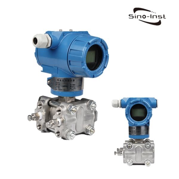
SI-702S Ultra High Pressure Transducer

Up to 1500 MPa | 0.25% accuracy | 4–20 mA — for hydraulic test rigs and ultra-high-pressure research.

FAQ

What is the output of a piezoelectric pressure sensor?

A raw piezoelectric crystal outputs a charge in picocoulombs proportional to the applied force. After signal conditioning, the field-deliverable output is a voltage (0–5 V or ±5 V common) for IEPE sensors, or a charge that an external charge amplifier converts to voltage for charge-mode sensors. Some integrated designs offer a 4–20 mA loop output, but only over their dynamic bandwidth.

Can a piezoelectric pressure sensor measure pull (tension) force?

Yes, but only if the crystal is mechanically preloaded. The preload puts the sensor in compression at rest, so a tensile force reduces the compression rather than reversing the sign. Without preload, a single crystal slice produces opposite-polarity charge under tension, and the diaphragm coupling typically prevents tension transfer altogether. Specialized force washers and load cells use this preload technique for tension and compression on the same channel.

How does a piezoelectric sensor differ from a piezoresistive one?

The names share a Greek root but the physics are unrelated. A piezoelectric sensor generates its own charge from a crystal under stress and only responds to changes in pressure. A piezoresistive sensor uses a Wheatstone bridge of silicon resistors whose resistance changes with strain; it needs an excitation voltage and reads true static pressure. Use piezoelectric for fast dynamic events; use piezoresistive for steady or slow process pressure.

Why don’t we use piezoelectricity for power generation in a serious way?

The energy density is very low. A square centimeter of PZT under modest stress produces microwatts. Useful sensing ranges down to femtowatts, but useful power generation needs orders of magnitude more, which would require either huge crystal areas or extreme stress amplitudes that fracture the material. Piezoelectric harvesting works for milliwatt-class wireless sensor nodes, not for replacing batteries or grid power.

Need Help Selecting a Pressure Sensor for a Dynamic Application?

Tell us the pressure range, frequency content, mounting interface, and process temperature. Our engineers will recommend a charge-mode or IEPE configuration with the right material and thermal protection. Most replies are sent within one working day.

Request a Quote

Please enable JavaScript in your browser to submit the form

What Is a Flow Transmitter? Working Principle, Signal Output, and How It Differs from a Flow Meter

Updated 2026-05-09 by the Sino-Inst engineering team.

A flow transmitter is the field instrument that turns a flow measurement into a 4-20 mA, HART, Modbus, or pulse signal that a PLC or DCS can read — and that a SCADA historian then trends across the plant. It sits between a primary element (an orifice plate, a magmeter coil, a vortex bluff body, a Coriolis tube) and the control room. This guide explains what is inside a flow transmitter, how each signal output works, how the device differs from a plain flow meter, and the five spec-sheet numbers that decide whether a transmitter actually fits the loop.

Contents

The Role of a Flow Transmitter in a Process Loop

Picture a typical 4-20 mA loop in a chemical plant. A primary element — say, an orifice plate — sits in the line and produces a measurable physical effect (a pressure drop). A flow transmitter reads that effect, applies the calibration curve, and outputs a single proportional signal: 4 mA at zero flow, 20 mA at full scale. The control room receives that one wire pair and treats it as the flow value.

That is the practical definition. A flow transmitter is the part that does three jobs: it senses, it conditions, and it transmits. A bare flow sensor cannot drive a 1500-foot cable run to a marshalling cabinet. A 4-20 mA transmitter can, because the signal is a current, not a voltage, and is immune to wiring resistance up to the loop budget.

For a deeper view of how the loop carries the signal, see our guide on upstream and downstream straight pipe requirements, which covers the install conditions that decide whether the reading you transmit is even valid.

Inside a Flow Transmitter: Primary Element, Sensor, Transducer, and Output Stage

A complete flow-measurement chain has four stages. Each stage has a job, and changing one without considering the others is the most common reason a “calibrated” loop reads the wrong number.

  1. Primary element — the device in the pipe that creates a measurable effect. Orifice plate, venturi tube, magmeter electrodes, vortex bluff body, Coriolis tube, ultrasonic transducers. Each has its own physics.
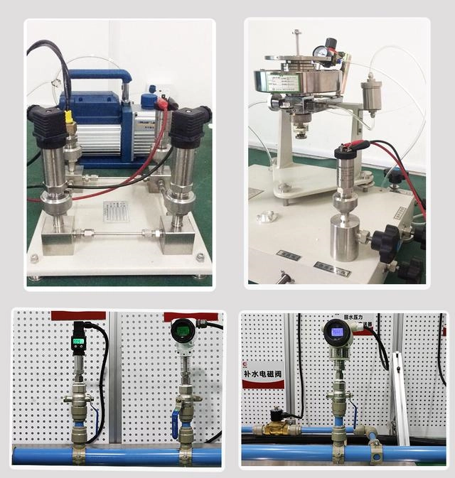
  2. Sensor — the part that reads the effect. A differential-pressure cell across an orifice. Two electrodes across a magmeter. A piezoelectric crystal behind a vortex bluff body. The sensor outputs a small electrical quantity (millivolts, microamps, picocoulombs).
  3. Transducer / signal conditioner — the analog and digital electronics that linearise, temperature-compensate, and scale the sensor signal into engineering units. This is where the calibration curve lives.
  4. Output stage — the transmitter proper. Drives 4-20 mA, encodes HART on top, talks Modbus RTU/TCP, or generates a scaled pulse output.

Take a magnetic flow transmitter as a worked example. The coils generate field B inside the meter body. Conductive liquid passing through cuts the field at velocity v, and Faraday’s law gives an induced EMF: V = k · B · D · v, where D is the bore diameter. That induced voltage is in the millivolt range. The transducer amplifies it, removes 50/60 Hz noise, applies the calibration K-factor, and the output stage scales the result to a 4-20 mA current loop.

Signal Output Options: 4-20 mA, HART, Modbus, and Pulse

The output you pick is dictated by what the receiving system speaks. Most modern transmitters offer two or more options on the same hardware, but mixing them is non-trivial.

OutputTypical useWiringPractical limit
4-20 mA analogContinuous flow rate to PLC/DCS analog inputTwin shielded, up to ~1500 m at 24 V loopOne value per pair; ~0.05% reading resolution at ADC
HART (over 4-20 mA)Diagnostics + secondary variables on existing 4-20 mA wiringSame twin shielded; HART superimposes 1200 baud FSKSlow data rate; needs HART-aware host
Modbus RTU/TCPMultivariable digital data — flow + totalizer + diagnosticsRS-485 multidrop (RTU) or Ethernet (TCP)Up to 247 nodes per RS-485 segment
Pulse / frequencyTotalizing into a counter (custody transfer, batching)Open collector or scaled frequencyOne pulse = one volume unit; needs care for low flow rates

For batch control or custody transfer, pulse output is still the most defensible because the count is unambiguous. For instrumentation under modern asset-management software, HART is the path of least resistance — every modern handheld speaks it. See our note on converting a 4-20 mA loop to 0-10 V when the receiver is a legacy voltage input.

How a Flow Transmitter Differs from a Flow Meter

The two terms get used loosely. Strictly, a flow meter is a device that indicates flow rate locally — a rotameter with a glass tube and a float, a paddlewheel with a mechanical totalizer, a magmeter with a field LCD. A flow transmitter is the version that also outputs a remote signal. Many modern devices integrate both: a magmeter body with a digital display on the converter, plus 4-20 mA / HART / Modbus to the control room. The same hardware sells under either name depending on whether the brochure is aimed at a maintenance engineer or a control engineer.

The practical decision is not about the names. It is about whether the value needs to leave the field, and over which protocol. If you only need a local read for plant rounds, a basic flow meter is enough. If a PLC or DCS must log the value, alarm on it, or use it in a control loop, a transmitter is required. See flow totalizer vs flow meter for the related distinction between rate-only and totalising units.

Reading a Flow Transmitter Spec Sheet — Five Numbers That Matter

A spec sheet is a contract. Five numbers do most of the work; the rest is decoration.

  • Calibrated range and turndown — the ratio between the highest and lowest flow the device measures within accuracy. A magmeter at 100:1 turndown is honest from 0.3 m/s to 30 m/s. A DP transmitter at 10:1 is fine in a steady-state line, painful in a varying batch process.
  • Accuracy class — read whether it is “% of reading” or “% of span”. 0.5% of reading at 10% of span is 5x worse than 0.5% of full scale near zero. Vendors quote whichever number looks better.
  • Process and ambient temperature — separate ratings. The wetted body sees process fluid temperature; the electronics housing sees ambient. The lower of the two limits is the one that bites.
  • Output and protocols — confirm 4-20 mA loop voltage budget (typically 12-42 V), HART revision, and Modbus addressing. Do not assume; ask.
  • Hazardous-area certification — ATEX, IECEx, FM/CSA, and the gas/dust group. A transmitter rated Zone 2 will not be accepted by the safety case for a Zone 0 vessel headspace.

For installation context that affects what numbers you actually achieve in the field, see our differential pressure flow meter calculation guide and the flow units cheat sheet when reading a US-units brochure.

Industrial Magmeter Flow Meters

Conductive liquids, DN10–DN3000. 4-20 mA + HART, accuracy ±0.5% of reading, IP68 sub-DN200.

Vortex Shedding Flow Meter

Steam, gas, low-viscosity liquid. 4-20 mA / HART / pulse. Up to 426 °C process temp, no moving parts.

Wedge Flow Meter

Slurries, dirty / abrasive fluids. DP-based, 4-20 mA / HART, recoverable signal at low Reynolds number.

Flow Transmitter FAQ

How does a flow transmitter work?

A flow transmitter reads a primary element (orifice, magmeter, vortex, Coriolis) through a sensor, applies the calibration in a transducer, and outputs a 4-20 mA, HART, Modbus, or pulse signal proportional to flow rate.

What is the difference between a pressure transmitter and a flow transmitter?

A pressure transmitter outputs a signal proportional to gauge, absolute, or differential pressure. For fast dynamic events such as engine in-cylinder combustion or hydraulic pulsations, a piezoelectric pressure sensor is used instead. A flow transmitter outputs a signal proportional to flow rate. A DP-based flow transmitter combines a DP cell with a primary element and a square-root extraction stage.

What are the three types of transmitters used in flow measurement?

Differential-pressure (orifice, venturi, wedge), velocity (magmeter, vortex, ultrasonic, turbine), and mass-flow (Coriolis, thermal).

What is the purpose of a flow transmitter in a process loop?

To convert a measured flow into a control-room-readable signal that can be logged, alarmed, used in a PID loop, or fed into custody transfer at any distance from the field.

Get a Quote from Our Flow Engineering Team

Tell us your line size, fluid, expected flow range, and required output protocol. Our engineers will respond within one business day with a recommended transmitter, datasheet, and lead time.

Request a Quote

Please enable JavaScript in your browser to submit the form

Related: flow rate unit conversions.

Paperless Recorders for Industrial Measure & Control System

Paperless recorders are data loggers that record and trend measurement data over time — replacing strip-chart and circular recorders with a touchscreen, internal flash storage, and Ethernet/Modbus TCP/OPC UA export.

Sino-Inst supplies industrial paperless recorders with 4 to 64 universal-input channels (thermocouple, RTD, mV, 4–20 mA, 0–10 V, pulse). Models cover general-process duty (R7100), temperature-focused heat-treat / pharmaceutical service (R7600), and dedicated flow-totalizer applications (F3000X). 21 CFR Part 11 audit trail and AMS 2750E compliance options are available, with Modbus TCP, OPC UA, and MQTT for SCADA / MES integration.

Sino-Inst offers a variety of low pressure transducers for industrial pressure measurement. If you have any questions, please contact our sales engineers.

For the underlying control algorithm running inside this recorder, see our explainer on the PID controller working principle and Ziegler-Nichols tuning.

Description

The paperless recorder is an electronic instrument that samples industrial process signals through a 24-bit ADC, applies the standard linearization (IEC 60584 for thermocouples, Callendar-Van Dusen for RTDs, scaled engineering units for 4–20 mA), and writes the result to internal flash storage. Up to 64 channels per chassis with 3-way galvanic isolation between channel-channel, channel-power, and channel-comms.

Front-panel touchscreen for live trend, alarm history and configuration. Trend stored as a tamper-evident binary file plus CSV; signed-PDF export available for 21 CFR Part 11 batch reporting. Communications include Ethernet 10/100, Modbus TCP slave, OPC UA server, MQTT publisher, USB host, and RS-485 Modbus RTU.

Features of Paperless Recorder

  • Universal input: K/J/T/E/N/S/R/B thermocouple, Pt100/Pt1000 RTD, 4–20 mA, 0–10 V, ±100 mV, pulse 0.1 Hz–10 kHz.
  • 4 / 8 / 16 / 32 / 48 / 64-channel models — pluggable hot-swap input cards.
  • 24-bit sigma-delta ADC, 100 ms–1 s sampling, configurable per-channel storage interval.
  • 3-way galvanic isolation (channel-channel, channel-power, channel-comms).
  • 21 CFR Part 11 audit trail, AMS 2750E heat-treat, GAMP 5, IEC 61010-1 compliance options.
  • Communications: Ethernet, Modbus TCP, OPC UA, MQTT, RS-485 Modbus RTU, USB host/device.
  • Front-panel IP65 for wash-down food and pharmaceutical service.
  • 3.5" / 5.6" / 7" / 10.4" / 12" TFT touchscreen, 4 GB flash + SD card.

Specifications of Paperless Recorder

ParameterR7100 UniversalR7600 TemperatureF3000X Flow Totalizer
Channels4 / 8 / 16 / 32 / 648 / 16 / 322 / 4 (pulse + 4–20 mA)
Display5.6" / 7" / 10.4"7" / 10.4"5.6"
Memory4 GB + SD card4 / 8 GB + SD2 GB + SD
Sampling100 ms / 200 ms / 1 s200 ms / 1 s100 ms (pulse) / 1 s
Compliance21 CFR Part 11AMS 2750E + 21 CFR Part 11OIML R117 (custody)
CommunicationsEthernet, Modbus TCP, OPC UA, MQTTEthernet, Modbus TCP, OPC UAEthernet, Modbus TCP, RS-485
Power90–264 VAC / 24 VDC90–264 VAC / 24 VDC90–264 VAC / 24 VDC
Panel cutout144 × 144 / 144 × 288 mm144 × 144 / 288 × 288 mm96 × 96 / 144 × 144 mm
Front panel ratingIP65IP65IP65

Read more about: Common Units Of Pressure

Applications of Paperless Recorder

  • Heat-treat furnace AMS 2750E TUS — 9 thermocouples + 1 control = 16-channel R7600 with Class 1 calibration.
  • Pharmaceutical sterilizer / autoclave — 21 CFR Part 11 mode, F0 calculation, signed batch report.
  • Food retort cook-cool validation — 1-minute storage, F0 trend, IP65 wash-down front.
  • HVAC and energy monitoring — temperature + flow + pulse from kWh, Modbus TCP to BMS.
  • Boiler / CHP plant — steam temperature, drum level, fuel-flow trending.
  • Custody flow measurement — F3000X with density/temperature compensation, batch totalizer.

What is a paperless recorder?

The paperless recorder is a stand-alone process data logger that replaces a strip-chart or circular recorder. Where the older instrument drew an ink trace on paper as the chart wheel rotated, the paperless recorder samples the same inputs at 100 ms–1 s, displays the trend on a touchscreen, and stores the values to internal flash for compliance and audit retrieval.

The recorded data are written as a tamper-evident binary file plus a CSV companion. The binary is the legally defensible record (signed checksum); the CSV is the convenience export for spreadsheets. Trend data and configuration changes are timestamped against an NTP-synced clock so the audit trail satisfies FDA 21 CFR Part 11 and AMS 2750E requirements for pharmaceutical and aerospace heat-treat work.

How does a paperless recorder work?

The paperless recorder is built around an industrial microprocessor, a 24-bit sigma-delta ADC, RAM and flash storage, and a touchscreen front. Each input channel is multiplexed through the ADC at the configured sampling rate (typical: 1 s per channel for compliance work, 100–200 ms for combustion and compressor monitoring).

The microprocessor applies the appropriate linearization curve (IEC 60584-1 for thermocouples, Callendar-Van Dusen for Pt100/Pt1000 RTDs, scaled engineering units for 4–20 mA inputs), computes alarm logic (HiHi / Hi / Lo / LoLo with deadband and on-delay), and writes the storage-interval-averaged value to internal flash. On alarm, a burst-capture routine stores the full sampling-rate data around the event so post-incident analysis sees the raw waveform.

Q&A

Is a paperless recorder the same as a data logger?

Closely related but not identical. A data logger is typically a small standalone unit with battery power and limited inputs; a paperless recorder is panel-mounted, plant-powered, with a touchscreen, more channels, built-in alarms, and SCADA integration.

How many channels do I need for a typical heat-treat furnace?

AMS 2750E TUS (temperature uniformity survey) calls for 9 thermocouples on a 60-225 cubic-foot furnace plus the control thermocouple – 10 channels active. Allow one card-slot of headroom and pick a 16-channel R7100 or R7600.

What protocols are available for SCADA integration?

Modbus TCP slave is standard. OPC UA server, MQTT publisher, and Modbus RTU (RS-485) are option keys. USB host accepts a flash drive for ad-hoc CSV export; Ethernet web server allows browser-based trend download.

Do paperless recorders need calibration?

Yes – annually for compliance work, every 2 years for non-critical applications. Calibration is per channel and includes the cold-junction reference for thermocouple inputs. Field calibrators (Fluke 754, Ametek MC) inject known signals and write the verification result to the audit trail.

What if I lose power mid-batch?

Internal flash memory is non-volatile, so the recorded data up to the power-off instant is preserved. The recorder reboots and resumes; a power-loss event is logged in the audit trail. For absolute continuity, a small UPS or 24 VDC battery backup is the recommended add-on.

R7100 Universal-Input Recorder

4 to 64 channels, universal input (TC/RTD/mA/V), 7″ or 10.4″ touchscreen, 4 GB internal + SD, Ethernet + Modbus TCP.

R7600 Temperature Recorder

8 / 16 / 32-channel temperature-focused recorder. 24-bit ADC, 3-way galvanic isolation, AMS 2750E-ready trend export.

F3000X Flow Totalizer

Specialized flow-totalizer recorder: pulse + 4–20 mA input, density/temp compensation, batch totalizer, RS-485 Modbus.

Sino-Inst supplies paperless recorders globally — heat-treat, pharma, food, HVAC, boiler, custody flow.

Channel counts from 4 to 64. Universal-input cards. 21 CFR Part 11 / AMS 2750E compliance options. Modbus TCP, OPC UA, and MQTT for modern SCADA / MES / IIoT integration.

Sino-Inst is a Chinese manufacturer with a global distribution network. Paperless recorders are most popular in heat-treatment, pharmaceutical, food, HVAC, and boiler / CHP markets across North America, Europe, India, and Southeast Asia. Send your channel mix, panel cutout, communication protocol and certification target — our team will configure and quote within 24 hours.

Request a Quote

Please enable JavaScript in your browser to submit the form